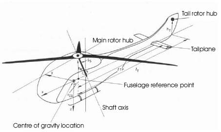
Figure 1. Helicopter Elements with Defined x, y, z axes Coordinate System [17]
This paper describes the mathematical modelling, analysis and simulation study of a helicopter with an external slung load system. The primary feature of the proposed model is the use of a helicopter model that consists of a six-degree of freedom, and combined with a three-dimensional motion load model. Considering the two models, a mathematical model for a helicopter carrying an external load is obtained. The combined system model can be used for stability analysis and controller development to improve flight handling quality and system performance. Stability analysis of the system was carried out via simulation. Simulation results revealed that the stability of the helicopter is significantly reduced due to the presence of an underslung load.
Due to its ability to carry large bulky loads externally on a sling, helicopters have become the most popular mode of transportation in many applications, such as large freight transportation, fire fighting and life saving missions. However, the external load can adversely affect the helicopter dynamics by the addition of further rigid body modes and aerodynamic forces that can seriously degrade the helicopter flight handling quality and reduce the operating envelop [1, 2].
The dynamics of a helicopter with an external suspended load received considerable attention since the late 70's and early 90's. This interest has been renewed recently, prompted by the re-evaluation and extension of the ADS- 33 [3] helicopter handling qualities specification to compact helicopters, and in the expectation of new cargo helicopter procurements [4]. Gubbles [5] investigated the effect of an external slung load on helicopter dynamics and handling qualities. The objective of that work was to compare helicopter dynamics and handling qualities for two cases. The first case involved an externally carried load on a single sling. The second case consisted of the same aircraft mass, with the load carried internally. Through this investigation the dynamic problems of carrying an external load on a sling were addressed.
The challenges of control of dynamics of a helicopter with an underslung external load are traditionally studied by means of simulations. The essence of flight simulation is in creating an illusion of reality for the pilot to experience. The quality or fidelity of this illusion will ultimately determine the boundary for what can and cannot be accomplished in terms of read-across to the real world. To demonstrate this fact, NASA has conducted both simulation and flight trials using UH-60 helicopter with an instrumented 8-by-6-by-6-ft cargo container [6-9].
A variety of literature has been published concerning various aspects of underslung load operations. Broader details of the subject can be found in various reports, which summarize the problems experienced in helicopters. These reports also suggest some technical solutions and analysis methods for some of the problems, see for example [10- 15]. In this paper, a study of dynamics of helicopters and the dynamics extended to helicopter with underslung external loads are carried out in order to gain insight into the dynamic characteristics of a helicopter with an underslung load. The analysis begins with the study of helicopter mathematical model, and then the development of a mathematical model of an underslung load, by considering the helicopter dynamics are the input to the load model is carried out in order to investigate the load dynamics. The work then proceeds to investigate the flight stability of the helicopter with an underslung load attached.Simulation studies have been performed using a simulation software. The results reveal how the stability of the helicopter is degraded by the influences of the load. The stability deceases as both the load weight and sling length are increased.
Dynamic model of a helicopter system may contain four interacting subsystems; main rotor, tail rotor, fuselage and empennage. In this paper a brief summary of a helicopter system dynamic model that is suitable for control study is presented. Details of the model can be found in [16].
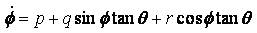
The helicopter has six degree of freedom in its motion and it has nine state variables in general, which are u,v,w the aircraft velocity components at centre of gravity, p,q,r, the aircraft roll, pitch and yaw rates about body reference axes, and θ,Ф,Ψthe Euler angles. To derive the equations of the translational and rotational motions of a helicopter, the helicopter is assumed to be a rigid body referred to an axes system fixed at the centre of mass of the aircraft, so the axes move with time varying velocity components under the action of the applied forces (see Figure 1[17]).
Figure 1. Helicopter Elements with Defined x, y, z axes Coordinate System [17]
The Euler angles define the orientation of the fuselage with respect to earth axes system [17, 18]. There are four control inputs, which are, longitudinal cyclic stick (η1s) lateral cyclic stick (η1c) collective lever (ηc) and pedal input (ηp) which control the helicopter's motion through X,Y,Z,L,M and N. So the system equations are as follows
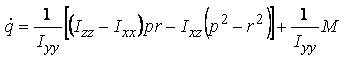
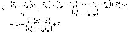
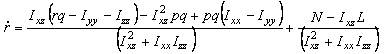
Where ma and g are the mass of the helicopter and a acceleration due to gravity, Ixx , Iyy , Ixx are the moment of inertia of the helicopter about x,y and z axes, and Ixz the aircraft product of inertia. The model (1) ~ (3) can be considered as a cascade connection nonlinear system, that is, it has the following form:

The overall external forces x, y, and z along x, y, z axes and moments L, M, N about x,y,z axes can be written as
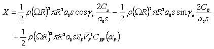
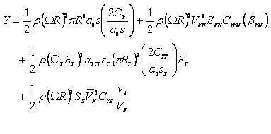
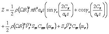
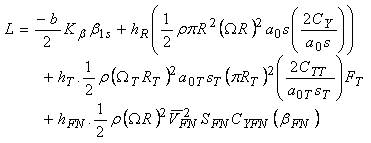
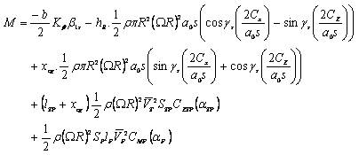
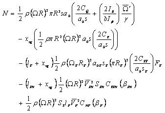
Where ρ is air density, R and Ω are the main rotor blade radius and speed, a0 and s the main rotor blade lift curve slope and solidity, and Cx , Cy , Cz Care the main rotor force coefficients in shaft axes.
A structure block diagram of a helicopter system from control point of view is shown in Figure 2. In Figure 2, downward arrows are used to indicate the flow of the system functionality. The flow of functions starts with the four control inputs, which are, longitudinal cyclic (θ1s) lateral cyclic (θ1c) collective (θc) and pedal (θ0T) which control the basic nine states of the system such as p, q, r, Ф, θ, Ψ, ν and w. The block diagram shows how the helicopter motion is achieved through the overall external forces XY and Z along x,y,x axes and moments L,M,N, about x,y,z, axes.
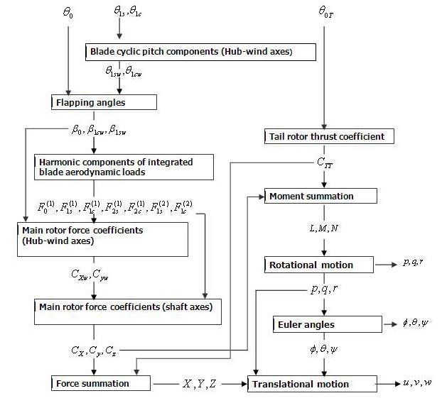
Figure 2. Structure Block Diagram of a Helicopter System
From the above description, it can be seen that the mathematical model is very complicated and nonlinear. Apart from simulation study, it is difficult to conduct any theoretic analysis based on this version of system model. In some cases, the simplified linear model may provide a helpful description to the helicopter to reveal some aspects of helicopter dynamics. So a linearised version of helicopter model is discussed in the next section.
The mathematical model presented in section 2 may be too complicated for analysis. Sometime it is necessary to make use of the well developed theory of linearisation to learn more about the behaviour of a nonlinear system [19]. Linearisation is an approximation in the neighbourhood of an operating point; it can only predict the local behavior of the nonlinear system in the vicinity of that point. In this study, the behaviour of the helicopter system at hover condition (operating point) is considered thus the linear model may be suitable for the analysis of a helicopter at a hover condition.
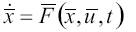
The helicopter equations of motion described in Section 2 can be written as follows
Where  = [Ф θ Ψ u v w p q r]T is the state variable vector,
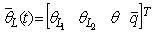
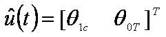
  =[θ1c θ1s θ0 θ0T]T is the control vector, and F represents the nonlinear relationship of the system state variables. To derive the linearised equations of motion using small perturbation theory, the helicopter behaviour can be described as a perturbation from the trim, written in the form

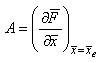
For linearization, it is assumed that the external forces X,Y and Z and moments L,M and N can be represented as analytic functions of the disturbed motion variables and their derivatives. Thus the forces and moments can then be written in the Taylor's expansion form. Then, the linearized equations of motion about a general trim condition can be written as in the state space  form and the system matrix A and control matrix B are derived from the partial derivatives of the nonlinear function
  i.e.
i.e.
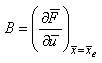
So the fully expanded form of the linear helicopter mathematical model has the following structure:
In order to investigate the longitudinal and lateral stability, the linear model can be reduced to longitudinal and lateral motion, by assuming that at hover trim condition, position, attitude and velocities are zero and longitudinal and lateral motion can be decoupled.
Decoupling longitudinal and lateral modes are common practices in the fixed wing aircraft, and the cross coupling derivatives would be zero. However, this is not the case for the helicopter as these cross-coupling terms influence the vehicle modes, and the handling qualities. But this decoupling or weakly coupled assumption leads to investigate the longitudinal and lateral modes separately as two distinctive sets. Phugoid, pitch and heave modes are identified as longitudinal modes and spiral, roll and dutch roll modes are identified as lateral modes [18].
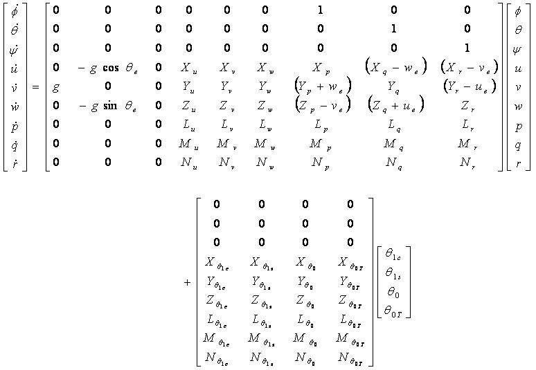
Equation of longitudinal motion
Where, longitudinal motion of the helicopter is uncoupled from lateral dynamics and described by four vector elements. It is assumed that the collective and (longitudinal) cyclic controls mainly influence the longitudinal motion.
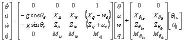
Equation of lateral motion
Where lateral motion of the helicopter is uncoupled from longitudinal dynamics and described by five vector elements. It is assumed that the pedal (tail rotor collective) and (lateral) cyclic controls mainly influence the lateral motion. Usually the heading angle Ψ is omitted from the matrices, as the direction of flight in horizontal plane has no bearing on the aerodynamic forces and moments [20]. Detailed discussion of state, control and stability derivatives of the matrices can be found in [18]. It discusses in detail some of their characteristics. The stability and control derivatives contained in the linear equations of motion aid in the understanding of helicopter flight dynamics. Analysis of the model takes place by considering that for small deviations from trim. The helicopter model can be determined from the system eigenvalues which are calculated from the stability matrix A.
To investigate the influences of a control input for a particular mission task, the state space representation can be transformed into a transfer function relationship between the states and controls. This is achieved simply by taking the state space representation.

and transforming it to the frequency domain to give
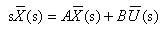
Finally, rearranging to relate the state variables to the control inputs gives
The helicopter handling qualities are strongly influenced by the stability of the normal modes, where stability of the mode is determined by whether or not the real part of the eigenvalue is positive or negative (stable modes having a negative real eigenvalue).
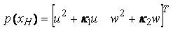
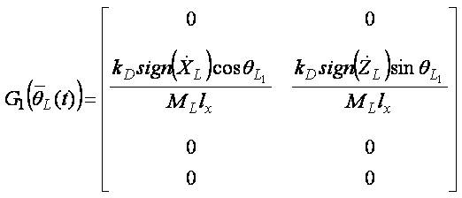
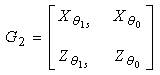
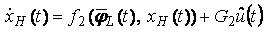
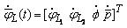
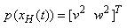
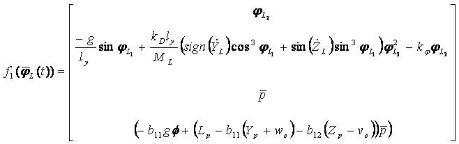
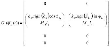
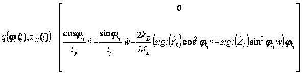
Helicopters with underslung loads have been the focus of significant interest in the aerospace research community for the last few decades' due to the inherent stability problems from which such systems suffer [10, 21]. The main contribution of this paper is to present a new approach to modeling a generic slung-load system that is in a general system point of view will have a structure of cascade connection of two subsystems. The specific focus for the model is simulation and controller design. The derivation of the model is based on combined modeling approach using a structure of cascade connection of two subsystems [21]. With this arrangement for the longitudinal motion of the helicopter with under-slung load combined system model can be written as follows;

Where,
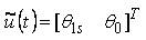
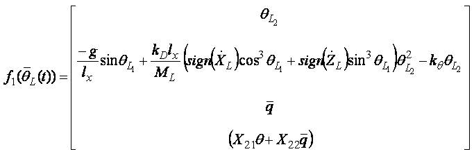
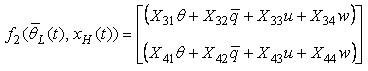
It is assumed that the longitudinal motion is primarily controlled by longitudinal cyclic commands (θ1s) and main rotor collective θ0
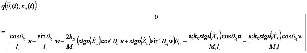
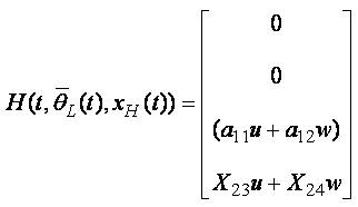
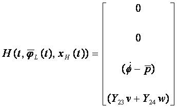
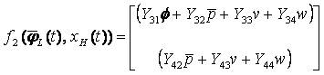
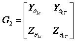
The helicopter with underslung load for lateral motion in the Y-Z plane can be described by the following equations;

Where,
It is assumed that the lateral motion is primarily controlled by lateral cyclic commands (θ1s)and the tail rotor collective θ0T.
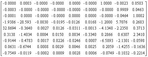
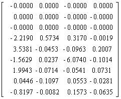
The helicopter model is linearised with reference to a standard nine state linear helicopter mathematical model [20]. Simulation softwares provide a tool to perform the task of system linearization. This is achieved by applying small perturbation to the state of the system, executing the simulation model, and then averaging the resulting partial derivatives over one revolution of the helicopter rotor. This procedure was performed for the cases both with and without an underslung load. The linearised system is expressed in the state space description form,  and the system stability was assessed by examining the location of the system poles on a root-locus diagram [22]. Using the simulation software's, the linearised model is obtained with the following state and input matrices.
In the case of, with an underslung load, the simulation model contains four more state variables which are, the longitudinal and lateral suspension angle position and the movement of angle position due to the two degree of freedom of suspension angles. The numerical values vary with respect to the sling- load configuration. It may represent the system dynamic variations. To investigate the stability characteristics of dynamic variations two series of simulation studies were carried out. Firstly, the sling length was kept at a constant and the load varied between the limits 500~2000lb. The corresponding root loci are sketched in Figure 3. Secondly, the load was kept at a constant and the sling length varied between the limits 10~20ft, to see the effect of varying the sling length.
Each of the diagrams shown in Figure 3 can be enlarged to view the pole locus near to Re(pole)=0 axis to demonstrate the variation of the system poles and to show that the positions of the system poles crossed the imaginary axis as the load weight increased and the whole helicopter system becomes less stable. For example considering the case of fixed sling length of 10 ft and 15ft with different load weights, the enlarged view of poles locus near to Re(pole)=0 axis are shown as in Figure 4 and Figure 5 with the resulted system poles listed in Tables 1 and 2. It is clear from the figures and system poles tables that the whole helicopter system becomes less stable when the load increases. The linearised helicopter model without carrying a load has system poles located on the left hand side of splane but near to the imaginary axis, which indicates that the system is stable but it may have strong oscillations in its dynamic responses and it is not very robust. The pole locus also indicates that the system (helicopter with load) poles have variation trends of moving further towards to right direction on the s-plane with increase of load weights.
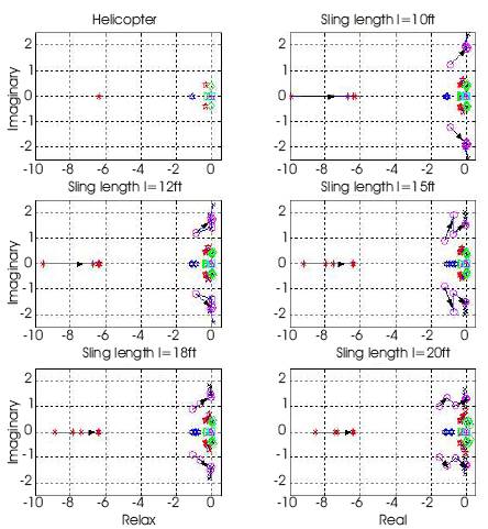
Figure 3. System Root-Locus Diagram Showing Pole Locus for Constant Sling Length as Load Weight is increased
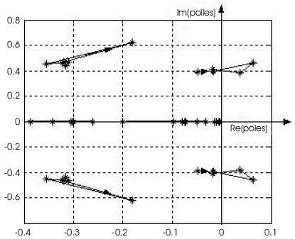
Figure 4. Enlarged View of the Case of Fixed Sling Length of 10 ft of Figure 3 Showing Poles Locus near to Re(poles)=0 axis
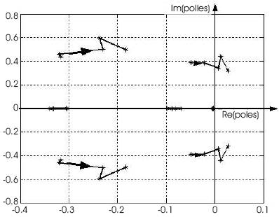
Figure 5. Enlarged View of the Case of Fixed Sling Length of 15 ft of Figure 3 Showing Poles Locus near to Re(poles)=0 axis
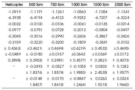
Table 1. System pole locations at sling length l =10 ft
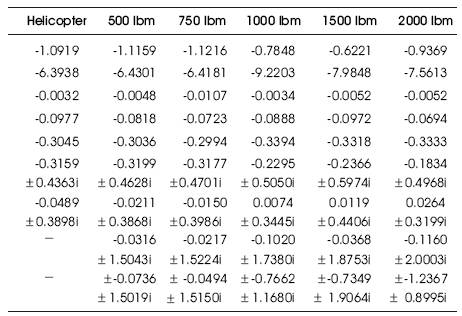
Table 2. System Pole locations at sling length l =15 ft
For Case II the load weight was kept at a constant and the sling length varied between the limit of 10 ~ 20 ft. The results of variation of the system poles and the corresponding root loci are illustrated in Figure 6. In Case 2, each of the diagrams shown in Figure 6 can be enlarged to view the pole locus near to Re(pole)=0 axis to demonstrate the variation of the system poles and to show that the positions of the system poles crossed the imaginary axis as the sling length increased and the whole helicopter system becomes less stable. For example considering the case of fixed load weight of 500 lbm and 1000 lbm with different sling lengths, the enlarged view of poles locus near to Re(pole)=0 axis can be shown as in Figure 7 and Figure 8, with the resulted system poles listed in Table 3 and 4.
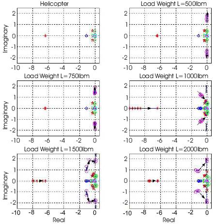
Figure 6. System root-locus diagram showing pole locus for constant load weight as Sling length is increased
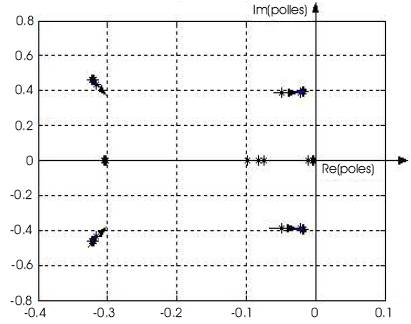
Figure 7. Enlarged view of the case of fixed load weight of 500 lBM of Figure 6 showing poles locus near to Re(poles)=0 axis
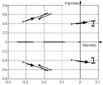
Figure 8. Enlarged view of the case of fixed load weight of 1000 lbm of Figure 6 showing poles locus near to Re(poles)=0 axis
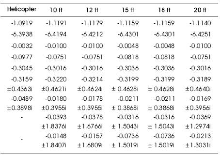
Table 3. System pole locations as load weight M = 500 lbm
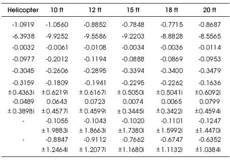
Table 4. System pole locations as load weight M = 1000 lbm
From the simulation results, it is evident that the stability of the helicopter can be significantly affected due to the presence of an underslung load. Analysis using a linearised system model shows that the helicopter-load combination becomes increasingly unstable as the load weight or sling length increases, which are revealed by the migration of the system poles towards the right hand side of the complex s-plane. The analysis shows how the stability of helicopter is affected by the influences of the addition of the underslung load. However, It is important to point out that the linearised helicopter model is only an approximation to the true system, furthermore in the process of linearisation rotor dynamics are ignored and only the six degree of freedom ridged body dynamics are considered. These results could be improved, if rotor dynamic and other factors affecting the helicopter dynamic such as unsteady aerodynamic are taken into account. Thus, this analysis provides the basis for a further analysis of stability of the system.
This paper presents modeling and simulation study of a helicopter with an external slung load system. Firstly, a generic mathematical model of a single main rotor helicopter is presented. The forces and moments that form the different elements of helicopter are discussed in detail. Secondly, studies on helicopter dynamics with an external under-slung load are carried out and a helicopter with an under-slung load system model has been derived. The model can be used for stability analysis and controller design.
Stability analysis of the helicopter with an external underslung load system was carried out via simulation. From the simulation results, it is evident that the stability of the helicopter can be significantly reduced due to the presence of an under-slung load. Analysis using a linearised system model shows that the helicopter-load combination becomes increasingly unstable as the load weight or sling length increases, as revealed by the migration of the system poles towards the right hand side of the complex s-plane.