The Inverted pendulum system is a favorite experiment in control system labs (Haiquan Wang, et al., 2013). The inverted pendulum system is characterized as typical high order, multivariable, unstable, non-linear system (Wang Luhao, and Sheng Zhanshi, 2010). They are typically used to realize experimental models, validate the efficiency of emerging control techniques and verify their implementation (Boubaker, 2012). It has many practical applications from Segway, human walking, humanoid robots to missile and rocket launchers. So, it is of great significance to study this system, both theoretically and practically. The inverted pendulum system is mounted on a movable cart. The track position and input voltage increase the complexity of the design. The system becomes more complex as the number of links increase.

There are various types of pendulum such as, the simple inverted pendulum, the rotary inverted pendulum, double inverted pendulum, and the rotary double inverted pendulum (A.G. Aribowo, et al., 2007). A lot of contributions exist in the stabilization of various types of inverted pendulum system (K. Furut, 1984; Ling Wang, et al., 2014). In this paper, a triple link inverted pendulum mounted on a cart is considered, thus making the system more challenging. The TLIP system is a SIMO (Single input multi Output) system which is represented in state space form for easy analysis. First, a Linear Quadratic Regulator (LQR) with a degree of stability is used for stabilizing the TLIP system. The system performance is analyzed on the basis of choices of Q and R matrices. Then Observer-based LQR Controller is used and the performances are compared. The main aim of this work is to improve the overall performance of the cart TLIP system. The concept of stability, controllability, and observability are also discussed. Here an attempt is made to control the pendulum's angle and cart's position. Section 2 explains the mathematical modeling of the cart TLIP system, section 3 deals with the methodology to stabilize the TLIP system, section 4 with simulation results and section 5 with the conclusion.

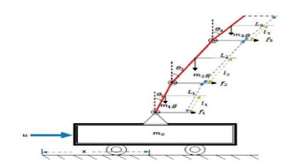
The mathematical model of the cart TLIP system is obtained by Lagrange method (Lijuan Zhang, and Yaqing Tu, 2006; Feizhou Zhang, et al, 1999). The schematic of the system is shown in Figure 1. The pendulum consists of three links of different lengths which are mounted on a cart; u is external action; x is the displacement of the cart; Θ₁ , Θ₂ , Θ₃ are the angles of the lower, middle, and upper pendulum bars respectively, with respect to the vertical line; m₀ is the mass of the cart; m₁ , m₂ , m₃ are the Centre masses of the lower, middle, upper pendulum bar respectively; L₁ , L₂ , L₃ are the length of the lower, middle, upper pendulum respectively. L₁ , l₂ , l₃ are the centroid of the lower, middle, upper pendulum bar respectively f₀ is the friction factor of cart and track, f₁ is the friction factor of lower pendulum and cart, f₂ is the friction factor of middle and lower pendulum, f₃ is the friction factor of middle and upper pendulum; J₁ , J₂ , J₃ are the rotary inertia of lower, middle and upper pendulum bar respectively, K_s is the overall system's input conversion gain (Mudita Juneja and Sheela Tiwari, 2014).

Figure 1. Schematic of Cart TLIP (Juneja and Tiwari, 2014

The generalized Euler-Lagrange equation is given as,

(1)

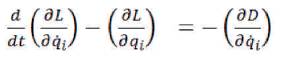
Where, Lagrange function (Lagrangian),

L = T – V,

T = Total Kinetic energy of the system,

V = Total Potential energy of the system,

W = Work done against friction (Dissipative forces),

q₁ , q₂ ……………, q_s are the generalized coordinates of the system.

The mathematical model of the triple inverted pendulum is constructed based on the Lagrange equations (C.J. Zhang, et al., 2012).

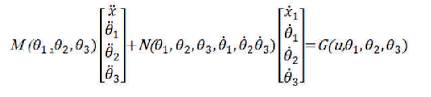
G₀ = [K_s 0 0 0]^T

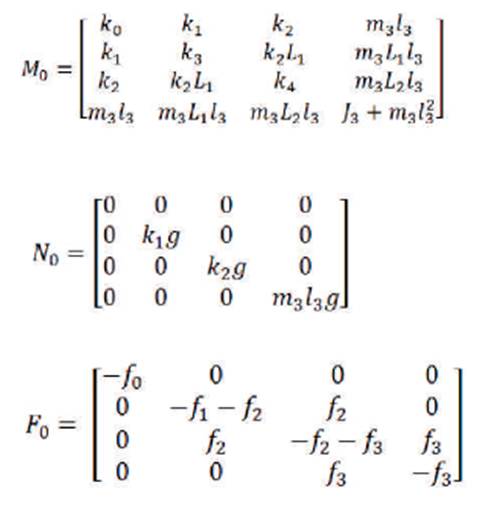
Where, the coefficients are given as:

(2)

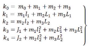
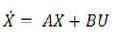
The linear model of the triple link inverted pendulum is represented in state-space form as follows:

(3)

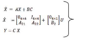
Where, A₂₁ = M₀^-1 x N₀ , A₂₂ = M₀^-1 x F₀ , B₂ = M₀^{- 1}x G₀

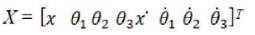
The state vector is defined by:

(4)

The coefficient matrices of state equation (3) of the cart triple inverted pendulum after putting the parameter values mentioned in Appendix are as follows:

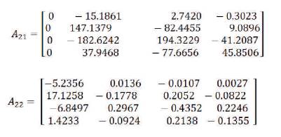
B = [ 0 0 0 0 3.7397 - 12.2326 4.8926 - 1.0166]^T

After obtaining the mathematical model of the system features, it is necessary to analyze the stability; controllability and observability of the system in order to further understand the characteristics of the system.

2.1 Stability Analysis

If the closed loop poles are all located in the left half of the s-plane, the system must be stable, otherwise the system is unstable. In MATLAB to strike a linear time invariant system, the characteristic roots can be obtained by eig (A, B).

The Eigen values of the system matrix A for the system are given in Table 1. The system is unstable as it has positive Eigen values. The model is simulated in MATLAB and the step response of the unstable open loop TLIP system is obtained as shown in Figure 2.

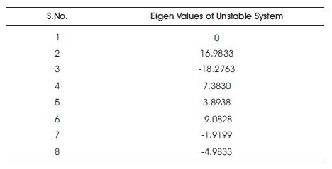
Table 1. Eigen Values of Open Loop System

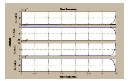
Figure 2. Step Response of Open Loop System

2.2 Controllability Analysis

C= [B AB A² B……. A^n-1 B],

Rank (C) =8

2.3 Observability Analysis

O= [C CA CA² ……CA^n-1] ^T

Rank (O) =8

Since it is proved that the TLIP system is controllable, a state feedback controller can be designed for making it stable.

3.1 The Design of LQR Controller with Degree of Stability α

For the cart TLIP system,

For this work, degree of stability α has been incorporated. All closed-loop poles are to the left of –α. In the controlled system described, the quadratic performance index cost function is given by,

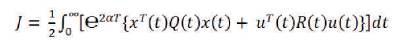
Where Q is a positive semi definite matrix, R is a positive definite matrix.

R = RT > 0, Q = QT ≥ 0, are weight matrices

u^*(t) = –K x(t)

K = R^-1 (t) B^T (t) P(t)

Where, K is the optimal feedback gain, P(t), a positive definite matrix is the optimal solution of matrix Differential Riccati Equation (DRE).

The Riccati matrix equation or Algebraic Riccati Equation (ARE) is given as,

PA + A^T P – PBR^-1 B^T P + Q = 0

Because of degree of stability α, the equation will be modified as follows:

P(A+ α I) + (A+ α I)^T P – PBR^{- 1} B^T P + Q = 0

In the design of the controller, one of the key problems is to select weight matrix Q and R in the quadratic performance indexes (Mukul K. Gupta, et al, 2014). If Q and R are selected not properly, a solution can be made that it cannot meet the actual system per formance requirements (Sandeep Kumar Yadav, et al, 2012). In general, Q and R are taken as the diagonal matrix, the current approach for selecting weighting matrices Q and R is simulation of trial. After finding a suitable Q and R, the optimal gain matrix K can be found easily.

First choosing Q matrix as Q = C*C^T

Q 1= diag ([1 0 1 0 1 0 1 0]), R=1 and Degree of stability α = 0.1

The optimal feedback gain matrix is

K= 1.0e+03 * [-0.0010 -0.0937 0.6301 -1.6867 - 0.0123 -0.0426 -0.0064 -0.1949]

The settling time and rise time are too large. To minimize the rise time and settling time, the value of the diagonal matrix Q are changed. This is done by iteration method. Replace the element of the matrix (Q) by,

Q2 = diag ([1400 1200 400 200 0 0 0 0]), R = 1, Degree of stability α=0.1

[K, P, E] = lqr (A, B, Q, R), where E is the open loop eigen value.

K2 = [-37.4166 -92.0858 349.1066 -536.1815 -47.0680 -15.8217 -7.4561 -90.3076]

From Table 2 it is clear that, the since all the Eigen values are negative the system becomes stable after using a LQR controller.

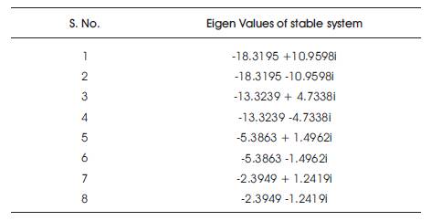
Table 2. Eigen Values of Closed Loop System

3.2 Observer based LQR Controller

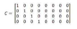
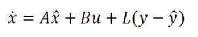
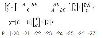
The response above was based on the assumption of fullstate feedback. We consider the situation where all state variables are not measured. In the TLIP system, only the cart position and the pendulum angle are directly measured. So a state estimator must be designed. This observer is simple in design and provides an accurate estimation of all the states. It is implemented by adding a correction term that is simply a gain on the error in the estimates. Before designing the estimator; the system under consideration should be observable. Since it is observing the dynamics of the state estimate are described by the following equation.

The last term corrects the state estimate based on the difference between the actual output and the estimated output . The dynamics of the error in the state estimate is given by,

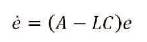
The error will approach zero if the matrix [A-LC] is stable, the speed of convergence depends on the poles of the estimator. Therefore the observer poles should be faster than the controller poles. Commonly estimator poles should be 4 to10 times faster than the slowest controller pole. The slowest poles have real part equal to -2.3949 therefore, placing estimator poles at -20. The statefeedback controller from before is combined with the state estimator to get the full compensator. The resulting closedloop system is described by the following matrix equations.

The step response of the cart TLIP system is shown in Figures 3 (a-d). From the above graphs it is clear that the system has become stable and now the settling time can be compared.

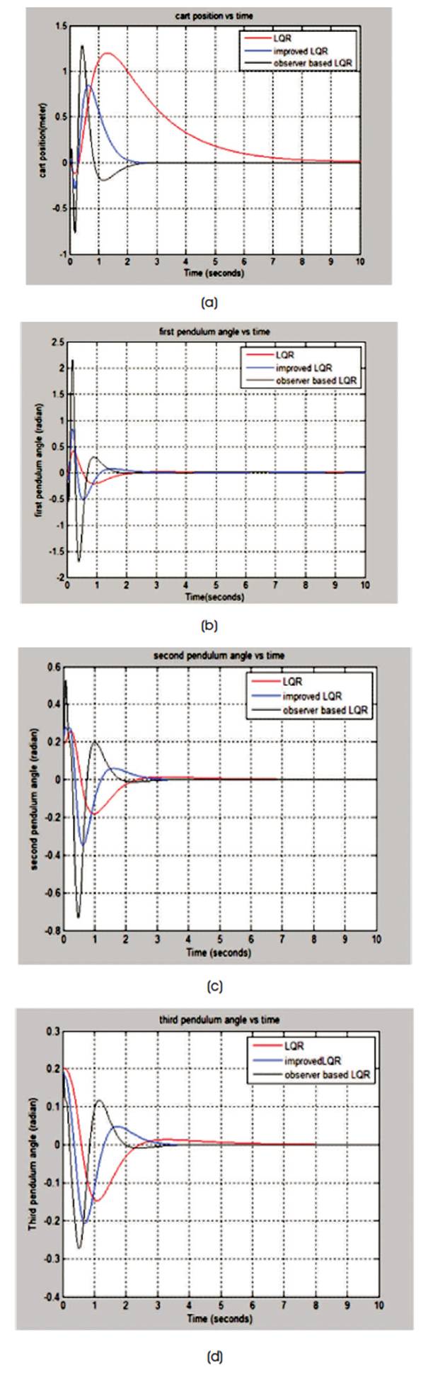
Figure 3 (a) Step Response of Cart Position, (b) Step Response of 1^st Angle, (c) Step Response of 2^nd Angle, (d) Step Response of 3^rd Angle

From Table 3, the improvement in settling time can be clearly observed. The settling time using Observer-based LQR Control for cart-position; first, second and third pendulum angles are 3.8%, 38.31%, 38.96%, and 6.9% less than LQR Control (Q2) respectively. The settling time gets significantly reduced for Observer-based controller, thereby increasing the stability of the cart TLIP system.

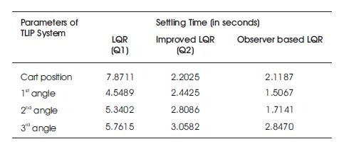
Table 3. Time Domain Specifications

This paper presents an optimal controller LQR to stabilize the cart TLIP system. The performance of the controller is found to be satisfactory as the settling time reduces. The steady state error is also obtained at zero. Based on the results obtained, the optimal controller is capable of stabilizing the cart position and pendulum angle of the TLIP system. The key problem in designing the LQR controller is selecting the weighting matrices Q and R. Advanced control algorithms for deciding the weighting matrices and use of intelligent controllers for stabilizing the TLIP system can be considered for future work.

m₀ = 2.4 Kg

m₁ = 1.323 Kg m₂ = 1.389 Kg m₃ = 0.8655 Kg

L₁ = 0.402 m L₂ = 0.332 m L₃ = 0.72 m

I₁ = 0.2449 m I₂ = 0.193 m I₃ = 0.3405 m

J₁ = .0119 Kg² J₂ = .0069 Kg² J₃ = .0291 Kg²

f₀ = 13.611 Nsm f₁ = .0045 Nsm f₂ = 0.0045 Nsm

f₃ = 0.0045 Nsm K_s = 9.722 NV g = 9.81 ms^{- 2}

(Sucheta Sehgal, and Sheela Tiwari, 2012).