Main role of Automatic Generation Control (AGC) is to maintain the system at their scheduled values during normal operating period [1]. The problem of controlling the real power output of generating units in response to changes in system frequency and tie-line power interchange within specified limits is known as Load Frequency Control (LFC). It is generally regarded as a part of Automatic Generation Control (AGC) and is very important in the operation of power systems [2].

The LFC is fundamentally for the problem of an instantaneous mismatch between the generation and demand of active power [3]. The objective of Load Frequency Control (LFC) is to minimize the transient deviations in these variables and to ensure their steady state values to be zero.

Mismatching between generated power and load demand leads to change in the frequency. In actual power system operations, the load is changing continuously and randomly, resulting in the deviations of load frequency and the tie-line power between any two areas from scheduled generation quantities. As technology has become so advanced that every system should work with stability and accuracy in order to get the efficient response, but at the same time due to complexity of systems and randomly changing load conditions, sometimes the stability could not be maintained. The fluctuation of load in these systems are very common, which can reduce their efficiency or may damage the system but it can be prevented by the use of different controllers in order to provide the automatic generation control or Load Frequency Control [4].

The most commonly used controllers are conventional I and PID controllers. The conventional PID control schemes will not reach a high of control performances [12]. Since the dynamic behaviour even for a reduced mathematical model of a power system is usually nonlinear and governed by strong cross-couplings of the input variables, special care has to be taken for the design of the controllers. For this reason, recently, a lot of artificial intelligence based robust controllers such as genetic algorithm, fuzzy logic and neural networks are used for PID controller parameters tuning in LFC.

Since, Particle Swarm Optimization algorithm is an optimization method that finds the best parameters for controller in the uncertainty area of controller parameters it has been used in almost all sectors of industry and science [11].

In recent years, most of the research is done in the aspect of different controllers in the area of automatic generation control for random load changes, but in this paper, a separate aspect of AGC is discussed [5]. This paper illustrates the effect of load parameter variations of two area power system in presence of conventional I as well as PSO-PID controllers.

It is observed that there is a lot of change in behaviour in the frequency response without controller and with controllers (I and PSO-PID) at fixed load parameters as well as variable load parameters. Simulations are carried out in MATLAB/ SIMULINK software. The transient responses of system with different controllers (I and PSO-PID) are compared to establish their effectiveness.

In the view of above, objectives of this work are as follow:

• To investigate the effect of load parameters variation on AGC of two area power system.
• To obtain better dynamic responses for AGC of two area power system with different load parameters.

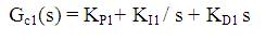
The control system that is used in this paper is two area power system [1]. The linearized model of the controlled system is shown in Figure 1 and system parameters are given in Appendix A. In the model, ΔP_L1 is step load  changes in area 1. Δf₁ is frequency deviation in area 1, Δf₂ is frequency deviation in area 2 and ΔP_tie is the tie-line power deviation. In two area system considered for study, the PID controllers with following structure is used.

(1)

(2)

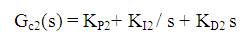
Where,

K_P is proportional gain

K_I is integral gain and

K_D is derivative gain respectively

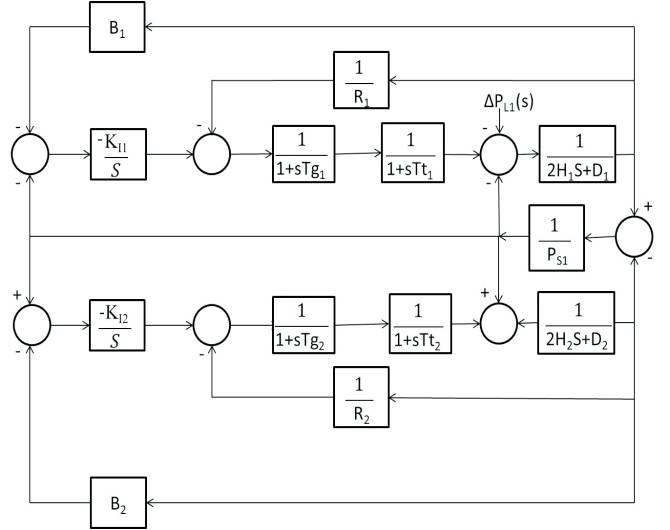
Figure 1. Linearized Model of Two Area System Model

2. PSO Algorithm

Particle Swarm Optimization (PSO) is a population (swarm) based stochastic optimization algorithm which was first introduced by Kennedy and Eberhart in 1995 [7]. It can obtain high quality solutions within shorter calculation time and stable convergence characteristics with PSO algorithm than other stochastic methods such as genetic algorithm.

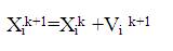
Particle Swarm Optimization uses particles which represent potential solutions of the problem. Each particles fly in search space at a certain velocity which can be adjusted in light of certain velocity, in light of proceeding flight experiences. The projected position of i^th particle of the swarm X_i, and the velocity of this particle V_i at (i+1) ^th iteration are defined by the following equations in this study [10].

(3)

(4)

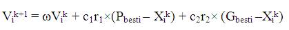
Where,

i=1,…... n and n is the size of the swarm,

c₁ and c₂ are positive constants

r₁ and r₂ are random numbers in [0,1],

k determines the iteration number,

P_besti represents the previous best of the ith particle ,

G_besti represents the best among all the particles in the swarm.

In this velocity updating process, the values of parameters such as ω, c₁ and c₂ should be determined in advance. In general, the weight ω is set according to the following equation (5) [8].

(5)

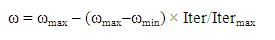
Where,

ω_max , ω_min initial and final weights,

Iter_max maximum iteration number

Iter current iteration number.

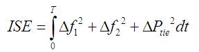
Main objective of the work is to minimize peak and settling time, so objective function is chosen as the Integral Square Error (ISE) [6].

(6)

The algorithm of PSO : [9]

• Initialize PSO parameters i.e., population size of the particles, no of iterations….etc.
• Select the control parameters, which values are need to be optimized.
• Evaluate fitness for each particle in the swarm
• Calculate P_best in N-dimensional space,
• Identify the particle which has the best fitness so far in N-dimensional search space, and assign its value to the G_best ,
• Update velocity and position of the particle using equations (3) and (4),
• Go to step 3 until optimized value is met.

At the end of the iterations, the best position of the swarm will be the solution of the problem i.e., G_best values will give optimal control parameters for PID controller.

In this proposed work, two area thermal power system have been developed by using Integral and PSO-PID controllers to illustrate the performance of load frequency control using MATLAB/SIMULINK software. Several types of Simulink models for different cases are developed with those controllers to obtain better dynamic behaviour. Frequency and tie-line power deviation plots for different parameter variations (D & ΔP_L ) are obtained as shown in figures.

3.1 Variable Load Damping Coefficient (D)

3.1.1 Case 1

In this case the dynamic response plots without any controller are given. Two area thermal power system as shown in Figure 2 is studied for variable load damping coefficient (i.e., D=0.1,0.6 & 3) and variable load change ΔP_L (10%, 30% & 50%) without any controller. Simulation results of frequency and tie-line power responses are given below.

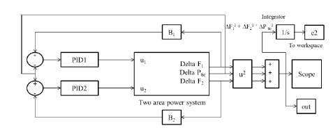
Figure 2. Implementation of PSO Algorithm for Two Area System.

a) Dynamic performances at load damping coefficient 0.1 are given below in Figures 3, 4 and 5.

b) Dynamic performances at load damping coefficient 0.6 are given below in Figures 6, 7 and 8.

c) Dynamic performances at load damping coefficient 3 are given below in Figures 9,10 and11.

Figures 3-11 show the dynamic responses for AGC of two area system without any controller, having different load parameters. To eliminate steady state error presented in dynamic responses, integral controller (I) is used. Dynamic responses with integral controller is given below.

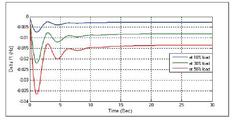
Figure 3. Change in Frequency Δf₁ without any Controller at D=0.1

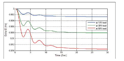
Figure 4. Change in Frequency Δf₂ without any Controller at D=0.1

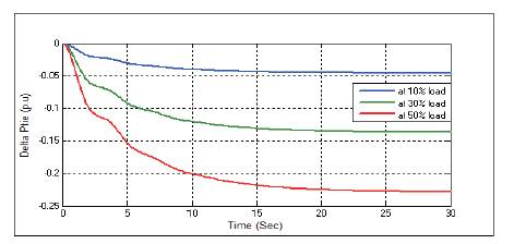
Figure 5. Change in Tie-line Power ΔP_tie Without any Controller at D=0.1.

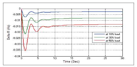
Figure 6. Change in Frequency Δf₁ Without any Controller at D=0.6

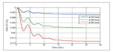
Figure 7. Change in Frequency Δf₂ without any Controller at D=0.6

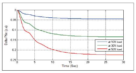
Figure 8. Change in Tie-line Power ΔP_tie Without any Controller at D=0.6

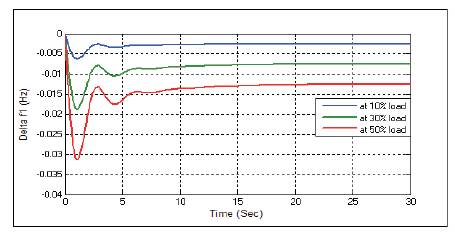
Figure 9. Change in Frequency Δf₁ Without any Controller at D=3

Figure 10. Change in Frequency Δf₂ Without any Controller at D=3

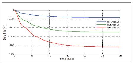
Figure 11. Change in Tie-line Power ΔP_tie Without any  Controller at D=3

3.1.2 Case 2

In this case the dynamic performance plots with integral (I) controller is analysed when one of the load parameter i.e. damping coefficient (D) is a variable (i.e., D=0.1,0.6 & 3) with variable load change ΔP_L , (10%, 30% & 50%) with integral controller. Simulation results of frequency and tieline power responses are given below.

a) Dynamic performances at load damping coefficient 0.1 are given below in 12,13 and14.

b) Dynamic performances at load damping coefficient 0.6 are given below in 15,16 and17.

c) Dynamic performances at load damping coefficient 3 are given below in 18,19 and 20.

Figures 12-20 show the dynamic responses for AGC of two area system in the presence of integral controller with different load parameters. To minimize the peak magnitude and settling time presented in dynamic responses, PSO tuned PID controller is used. Dynamic responses with PSO tuned PID controller is given below.

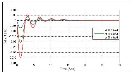
Figure 12. Change in Frequency Δf_L with Integral Controller at D=0.1

Figure 13. Change in Frequency Δf₂ with Integral Controller at D=0.1.

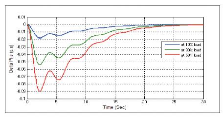
Figure 14.Change in Tie-line Power ΔP_tie with Integral Controller at D=0.1.

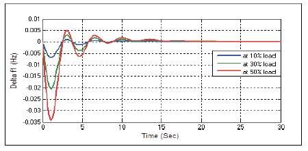
Figure 15. Frequency Response Δf₁ with Integral  Controller at D=0.6

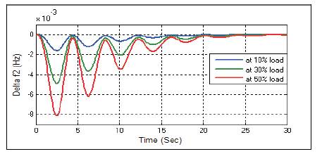
Figure 16. Change in Frequency Δf₂ with Integral Controller at D=0.6

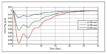
Figure 17.Change in Tie-line Power ΔP_tie with Integral Controller at D=0.6

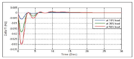
Figure 18. Change in Frequency Δf₁ with Integral Controller at D=3

Figure 19. Change in Frequency Δf₂ with Integral Controller at D=3

Figure 20. Change in Tie-line power ΔP_tie with Integral Controller at D=3

3.1.3 Case 3

In this case the dynamic response plots with PSO-PID controller is analysed when one of the load parameter i.e. damping coefficient (D) is a variable with variable load change ΔP_L .The simulation plots at different values of D (i.e.,D=0.1,0.6 and 3) with variable load change ΔP_L . (10%, 30% & 50%) with PSO-PID controller is studied. Simulation results of frequency and tie-line power responses are given below.

a) Dynamic performances at load damping coefficient 0.1 are given below in 21,22 and 23.

b) Dynamic performances at load damping coefficient 0.6 are given below in 24,25 and 26.

c) Dynamic performances at load damping coefficient 3 are given below in 27,28 and 29.

Figures 21-29 show the dynamic responses for AGC of two area system in the presence of PSO-PID controller with different load parameters. Dynamic responses for AGC of two area power system with PSO tuned PID controller having different load parameters offers minimum Peak magnitude and settling time.

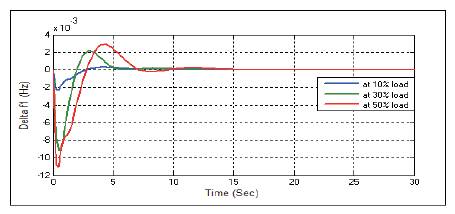
Figure 21. Frequency Response Δf₁ with PSO-PID Controller at D=0.1.

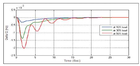
Figure 22. Change in Frequency Δf₂ with PSO-PID Controller at D=0.1

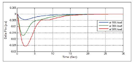
Figure 23. Change in Tie-line Power ΔP_tie with PSO-PID Controller at D=0.1

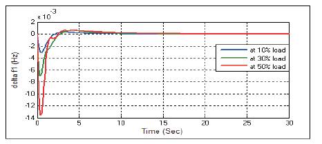
Figure 24. Frequency Response Δf₁ with PSO-PID  Controller at D=0.6

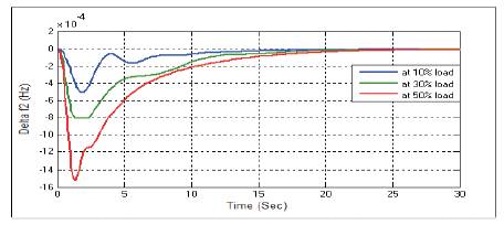
Figure 25. Change in Frequency Δf₂ with PSO-PID Controller at D=0.6

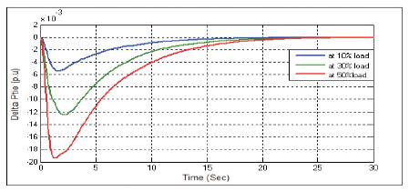
Figure 26. Change in Tie-line Power ΔP_tie with PSO-PID Controller at D=0.6

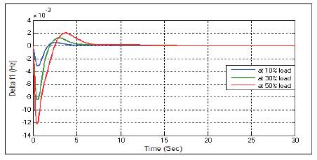
Figure 27. Frequency Response Δf₁ with PSO-PID Controller at D=3

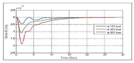
Figure 28. Change in Frequency Δf₂ with PSO-PID  Controller at D=3

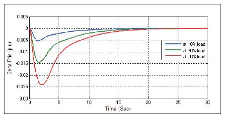
Figure 29. Change in Tie-line Power ΔP_tie with PSO-PID Controller at D=3

In this paper, PSO-PID has been investigated for load frequency control of a two area power system. For this purpose, first, to obtain the PID controller parameters, PSO algorithm is used. It has been shown that the proposed control algorithm is effective and provides significant improvement in system performance. Therefore, the proposed PSO-PID controller is recommended to generate good quality and reliable electric energy. In addition, the proposed controller is very simple and easy to implement since it does not require many information about system parameters.

In this work, load damping coefficient D and load change ΔP_L are taken as variables for variation of load parameters. The authors have taken the inertia constant H also as a variable for variable load parameter.

Appendix

System Data

F=60Hz, R1=0.05, R2=0.0625, D1=0.6, D2=0.9, H1=5, H2=4, Tg1=0.2sec, Tg2=0.3sec, Tt1=0.5sec, Tt2=0.6sec, Base power = 1000 MVA.

PSO algorithm:

Pop size = 10;

ω_max = 0.9

ω_min = 0.4

C_R = 0.65

c₁ = 2.0

c₂ = 2.0

iter_max = 30