For generations, it was a desire of humans to develop intelligent systems which can obey them from ground, in water and in the air. UAVs are one such development of aeronautical, instrumentation and control system technologies[1]. UAVs are of different sizes according to applications and have a wide range of civil and military applications such as remote sensing, environmental monitoring (e.g. pollution, weather, and scientific applications), forest fire monitoring, home land security, border patrol, drug interdiction, aerial surveillance and mapping, traffic monitoring, precision agriculture, disaster relief, adhoc communications networks, and rural search and rescue [2].

The main building block of UAV is automatic flight controller, also known as autopilot. This autopilot controls UAV by generating control signals on the basis of desired flight path, target information and waypoints. The various sensors are used in UAVs to generate feedback signals for the controller on the basis of real time state of the vehicle. The autopilot is controlled by a pilot on the ground or in another vehicle. A typical launch and recovery method of an unmanned aircraft is done by an automatic system or an operator on the ground [3]. The traditional approach used for flight control system synthesis, implementation and validation is time consuming and resource intensive. To make cost effective autopilots for these aerial vehicles computer technology plays an important role [4]. MATLAB is one such platform on which we can simulate and test the performance of an autopilot [5]. Conventional Proportional Integral (PI) and Proportional Integral Derivative (PID), state feedback controllers and robust fuzzy logic controllers can be used to make autopilots to track the desired flight path. In this paper, Proportional Integral (PI) controller based UAV is presented to control the lateral parameters of fixed wing UAV and hence to improve its tracking path performance.

Mathematical model of 6-DOF medium sized, fixed wing UAV is multivariable, time variant and non- linear in nature [6]. Understanding and solving such a plant is a very complex problem, so, conversion of non-linear model into a linearized model is the primary requirement for autopilot designing which provides clear insight into the system dynamics.

The nonlinear dynamic model of UAVs is developed with the help of force and moment equations. An aircraft has three linear and three rotational motions to compose its six degrees of freedom. Mathematical model used for medium sized unmanned aerial vehicle is given by Iftikhar H Makhdoom and Shi Yin Qin [7]. Its small perturbation linearized model is adapted to design autopilots to control UAV's angular velocity along X-axis, Yaw, Roll and Angular velocity along Z-axis. Laws of physics are applied on the vehicle to find mathematical differential equations. All the calculations are done by taking parameter values with respect to centre of gravity of vehicle. Force and moment depends on the thrust applied by engine and engine speed is taken in revolution per minute (rpm) [8].

To derive dynamics of UAVs, consider vehicle heading along x axis, its right wing and z axis downward, passes through its centre of gravity and perpendicular to both x and y axis. Suppose, the state vectors are in North East Down (NED) projection. By assuming flat earth model, the nonlinear dynamic state equations are [9-10].

(1)

(2)

(3)

(4)

(5)

(6)

(7)

(8)

(9)

(10)

(11)

(12)

Where X= [ p_N p_E p_D Φ θΨ U V W P Q R], [X_T , Y_A , Z_A] are  aerodynamic forces. These aerodynamic forces and moments depend on elevator, throttle, aileron and rudder actuator control vectors [δ_e,δ_t,δ_a,δ _r] and various other flight variables. The propulsive forces are represented by [X_T , Y_T ,  Z_r ] and [l, m, n] are moments.

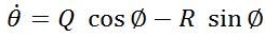
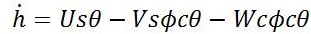
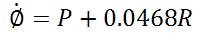
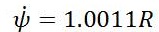
, where J represents the 3×3 inertia matrix, θ, Φ and ψ are the Euler angles (roll, yaw and pitch angles) and g_D is acceleration due to gravity in NED axis and h=-p_D with vehicle weight M. c Φ = cosΦ and SΦ=sinΦ are the other notations used in above equations.

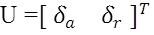
Linear model consists of longitudinal and lateral model of system. To control angular speed along X-axis, yaw and roll of vehicle we need only lateral model of the aircraft having five states and two inputs, Aileron and Rudder [11]. Aileron is used to control angular speed along X axis, yaw and roll of the aircraft while Rudder is used to control vehicle angular speed along Z -axis.

The performance of an aircraft can be described by assuming the aircraft as a point mass concentrated at the aircraft's center of gravity 'cg'. The flying qualities of an aircraft must, instead, be described analytically as motions of the aircraft's cg, motions of the airframe about the cg, both of which are caused by aerodynamics, thrust, other forces and moments[12]. So, the aircraft must be considered as a three dimensional body, and not a point mass. Various forces and moments on 6 DOF UAVs [13] are shown in Figure 1.

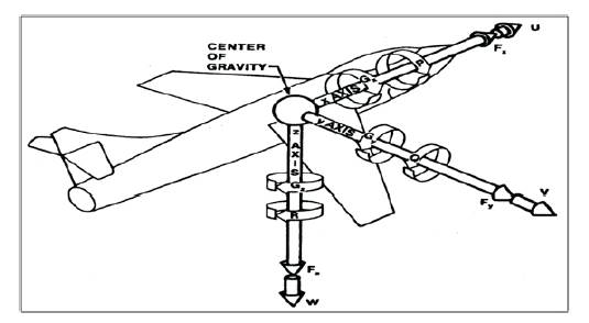
Figure1. Various Forces and Moments on a 6-DOF UAV [13]

The applied forces and moments on the aircraft and the resulting response of the aircraft are traditionally described by a set of equations known as the aircraft equations of motion. The equations that will be developed are not as rigorous and complicated as those are used for design of modern aircraft, but the basic method is valid and will provide analysis techniques that are accurate enough to gain an insight into aircraft flying qualities [14].

Decoupling of nonlinear equations is done by considering both bank angle and sideslip angle equal to zero which provide a normal flight condition and convert nonlinear set of equations into two sets for longitudinal and lateral motions of aircraft. Conversion of nonlinear equations into linear equations uses small perturbation theory at normal non accelerated flight at constant speed. Linear model can be found by using MATLAB commands around the trimmed conditions [10].

An aircraft has six degrees of freedom (if it is assumed to be rigid body), which means it has six paths, free to follow: it can move forward, sideways, and down; and it can rotate about its axes with yaw, pitch, and roll as shown in Figure 2.

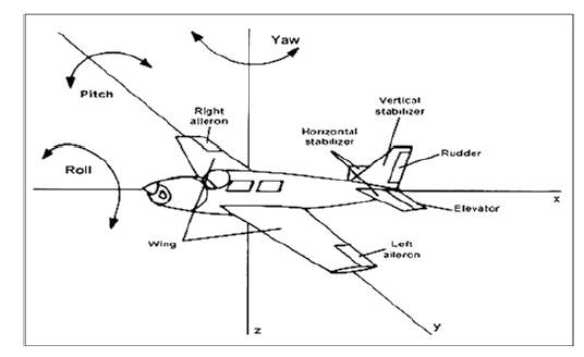
Figure 2. Various Motions and Controlling Parameters of UAV

Inorder to describe the state of a system having six degrees of freedom, values for six variables are necessary. To solve for these six unknown variables, six aircraft equations of motion are required. The full aircraft equations of motion reflect a rather complicated relationship between the forces and moments on the aircraft and the resulting aircraft motion.

1.2 State Space Equations of UAV

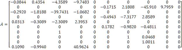
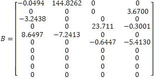
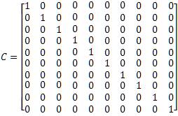
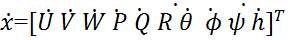
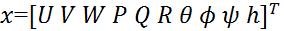
The nonlinear set of equations of aircraft dynamics can be linearized using MATLAB commands and linearized model can be easily converted into state space model. This linearization is done around a flight condition called as trim conditions of dynamic model. The linear model and its conversion into state space leads to selection of desired MIMO systems for the control of UAVs. State equations of medium sized fixed wing UAV are given as:

(13)

(14)

(15)

(16)

(17)

(18)

(19)

(20)

(21)

(22)

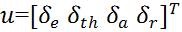
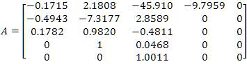
State space model of any plant can be given as:

(23)

(24)

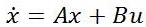
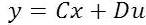
Where states outputs u, y represent inputs and output respectively. A, B, C and D represent state, input, output and direct transmission matrices respectively. These can be easily calculated from the state equations of the vehicle.

(25)

(26)

(27)

(28)

Where;

(29)

(30)

(31)

1.3 State Matrices for Lateral Dynamics

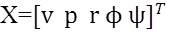
As said above, the whole system is divided into two subsystems, Longitudinal and Lateral. The state space model for Lateral subsystem is given as:

(32)

(33)

(34)

(35)

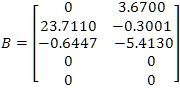
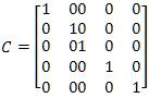
Where:

(36)

(37)

2.1 Simulation and Response of Open Loop Lateral Subsystem

Open loop Lateral subsystem is designed by considering various input-output transfer functions and their simulation on MATLAB[15] platform. The simulink model of open loop lateral subsystem is shown in Figure 3. Step signal is taken as input signals for Aileron and Rudder, whereas the responses of UAV are lateral parameters i.e., angular speed along xaxis, yaw, roll and angular speed along z-axis which are shown in Figures 4, 5, 6 and 7 respectively.

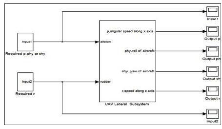
Figure 3. Simulink Model of Open Loop UAV Lateral Subsystem

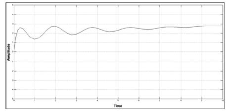
Figure 4. Angular Speed of UAV Along X axis

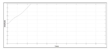
Figure 5. Output Ø(Roll) of UAV

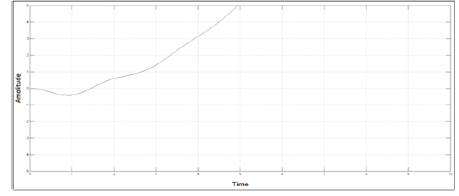
Figure 6. Output (Yaw) of UAV

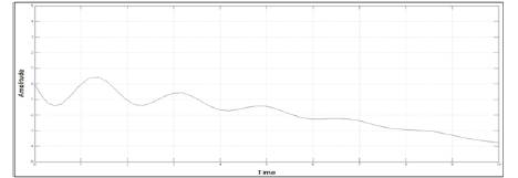
Figure 7. Output r(angular velocity along Z axis) of UAV

2.2 Closed Loop Control of Lateral Parameters of UAV

In this paper, lateral parameters of UAV are controlled by using PI controller. Lateral Autopilot consist of three PI controllers [16,17] i.e, one controller for the control of angular speed along x-axis, second controller for yaw and roll control and third controller for the control of angular speed along z-axis. The major task for lateral parameter control of UAV is the control of Aileron deflection for height control and the control of Rudder for speed control. The guidance block of the vehicle generates commands based on the required trajectory for lateral parameters. These control objectives are achieved by converting MIMO system into Single Input Single Output (SISO) system [18].

Control of yaw and roll is done by applying multiple feedback loops and control of angular speed along x-axis and z-axis is done by individual feedback loops [19,20].

2.3 Simulation and Response of Closed Loop PI Controlled UAV

Simulink models for the control of lateral parameters of UAV using PI controllers are shown in Figures 8 and 9 respectively. In this paper, unit step signal is taken as set point value and Controller gains (k_p and k_i, proportional  controller and integral controller gain respectively) are calculated by Tyreus-Luyben tuning method [21]. The ultimate Gain and frequency of open loop system which can be used to calculate controller gain, are calculated using root locus plot. Many other methods are also available now a days for effective controller tuning [21-23]. Controller's gain for the expectable outputs of system with minimum overshoots and steady state errors are summarized in Table 1.

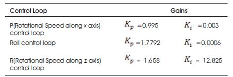
Table 1. PI Controller Gains for Lateral Parameters Control

The simulated responses of UAV for different lateral parameters are shown in Figures 10, 11, 12 and 13 respectively.

Figure 8. Simulink Diagram of PI Controlled UAV for Sideslip p (angular velocity along X axis) and r (angular velocity along Z axis)

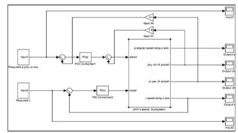
Figure 9. Simulink Mmodel of PI Controlled UAV for Roll Angle r (angular velocity along Z axis)

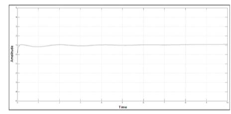
Figure10. Response of PI Controlled UAV for p (angular velocity along X axis)

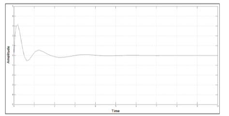
Figure 11. Response of PI Controlled UAV for Output of (Yaw)

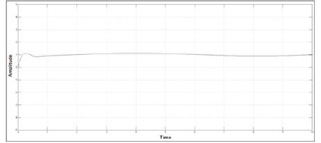
Figure 12. Response of PI Controlled UAV for Output

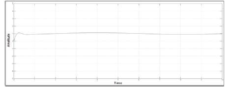
Figure 13. Response of PI Controlled UAV for Output r (angular velocity along Z axis)

In this paper, a flight control design technique for the lateral parameter control of UAV is presented. This paper simplifies the non-linear model of UAV by linearization and then converts MIMO system into simple SISO systems. Lateral Autopilot is designed for a given flight conditions, this design technique can be repeated for a series of flight conditions. Keeping control objectives i.e minimum overshoots and steady state errors in mind, multi-loop control technique and simple feedback control techniques are applied. PI controllers are used to achieve control objectives. As seen from the open loop response shown in Figures 4, 5, 6 and 7 and closed loop PI controlled UAVs response shown by Figures 10-13, a substantial improvement in lateral parameters of UAVs has been achieved.