Figure 1. The Study Area and its Associated Villages
The K means clustering was processed for threshold vegetation indices and gap detection. It was processed for retrieving the vegetation index value that represents forest land cover, percentage vegetation coverage, and canopy density. The method was further used for finding the probability distribution of forest canopy gaps in the forest. The result was tested in the Hazaribagh Wildlife Sanctuary, Jharkhand, India. The percentage vegetation cover was calculated in the new SNAP software. The canopy density was mapped through FCD model. From the analysis, it was estimated that the dense forest having greater than 70% of canopy density comprises 64-100% of vegetation cover; moderately dense forest having 40-70% canopy density includes 21-64% of vegetation cover, and open forest having less than 40% canopy density have 7-21% of vegetation cover. The Normalized Vegetation Index (NDVI) and Transformed Vegetation Index (TVI) considered being more efficient and Difference Vegetation Index (DVI) was less efficient for forest vegetation cover and density measurement. Inversely, it was observed that DVI was more efficient in finding gaps in the forest. The method was also functional for finding the probability distribution of canopy gaps in the forest. This clustering technique can be applied in other means for forest landscape level assessment.
Many previous works established the classification of images like (Matsuyama, 1987) provides use of Artificial Intelligence (AI) techniques for remote sensing (Blonda et al., 1991) reported that a rule-based fuzzy logic approach gave better results than a maximum likelihood classifier on a multi temporal data set. K-means, a simple and effective clustering unsupervised classification algorithm and one of the most widely used clusters in the classification of images (Wang et al., 2015). The K-means algorithm divides M points in N dimensions into K clusters to perform the overall classification (Hartigan & Wong, 1979). It has many applications, especially in land cover classification. Many types of research demonstrated how such information can be useful for understanding the status of a forest and remote sensing can provide new standpoints and potentials for forest cover monitoring.
Remotely sensed spectral indices were prime source of knowledge for the monitoring of vegetation character and number of Vegetation Indices (VIs) developed in the past few decades which are spectrally defined and has the ability to quantify vegetation properties. Most of the vegetation indices are calculated from a mathematical formula which contains red and NIR bands as input. Vegetation indices are numerical measurements representing the vigor of vegetation (Campbell & Wynne, 2011). It is with great effort to identify which indices can be used for specific purposes. The usefulness of vegetation indices is immense that help in land use and land cover changes monitoring, forest cover, canopy density, crop prediction, and discrimination analysis (Baret et al., 1986). They do not have a standard universal value and research often shown different results.
The present study utilizes the Forest Canopy Density model (FCD) developed by the International Tropical Timber Organization (ITTO) (Rikimaru et al., 2002; Rikimaru, 1997). The model requires many vegetation indices and integration of it to get canopy density, which can be further utilized for other forest analysis. Dense forest having a high canopy density speaks about the good health of the forest while light or no coverings show the inverse. It is made to be used for Landsat TM data, but in the study, the forest canopy density was calculated from sentinel-2 imagery. With the help of canopy density forest classes like a dense forest, moderately dense forest, open forest, degraded forest, and non-forest can be defined. The good thing about this model is that it requires less ground truthing and accuracy assessments.
Forest canopy gaps are too large for manipulative experiments to be readily undertaken, and hitherto grassland gaps have been too small to be easily mapped (Silvertown & Smith, 1988). The spatial properties of gaps have an important influence on the regeneration dynamics and species composition of forests. Using field measurements for delineation of gaps is very challenging for a vast area. This problem can be solved by considering and measuring it from the remote sensing point of view.
The imagery of Sentinel-2 having a spectral resolution of 10 m and utilizing red and NIR bands make the calculation of used vegetation indices in the present study. The several studies have been implemented that show the potential of Sentinel-2 for measuring many biophysical and biochemical parameters such as Leaf Area Index (LAI), chlorophyll content and product such as a red edge position index (Van der Meer et al., 2014).
The objective of the present study is to use vegetation indices like Ratio Vegetation Index (RVI), TVI, DVI, and NDVI for finding its threshold on forest land cover, Percentage Vegetation Cover (PVC) and canopy density mapping. Then, utilizing it for forest canopy gap identification and finding the probability of gap occurrence.
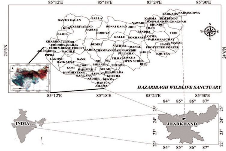
The present study was conducted in the Hazaribagh wildlife sanctuary, Jharkhand, India (Figure 1). It lies between 24°45'22” N to 24°08′20″N latitudes and 85°30'13” E to 85°21′58″E longitudes.
Figure 1. The Study Area and its Associated Villages
The present study used high-resolution ESA Sentinel 2A data acquired on 2016/02/13 (Addabbo et al., 2016) (Table 1) and the data were subset to the area of Hazaribagh Wildlife Sanctuary. The images were processed with Wgs 84 datum projection system using nearest neighbor resampling. The data were cloud free and acquired from Earth explorer (http://earthexplorer. usgs.gov). The methodology adopted is given in Figure 2 (Drusch et al., 2012).
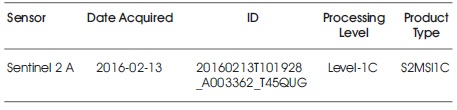
Table 1. Satellite Data used in the Present Study
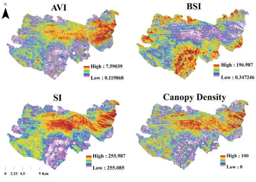
Figure 2. The Indices used for Forest Canopy Density Modelling and Canopy Density Estimation in the Study Area
The present examination is based on the reflectance properties of bands on Sentinel 2A satellite data for the estimation of radiometric vegetation indices. The imageries require atmospheric adjustment and alignment before their handling. For this reason, the raw satellite imagery of Sentinel 2A was firstly converted into reflectance. The DN (Digital Number) to reflectance conversion (Calibration) needs a header document given in the downloaded satellite imagery, which contain all the necessary inputs for correcting the imagery like acquisition date, sun height, gain, and bias (Lv et al., 2010). Then, the images were corrected by the Dark Object Subtraction (DOS) to get real surface reflectance of the object. The DOS strategy is an image based technique to counterbalance the haze component caused by additive scattering from remote sensing data. Quantum GIS (QGIS) Software was utilized in the pre-preparing of the Sentinel 2A imageries. It incorporates the element of programmed transformation of DN to reflectance by utilizing a header record and DOS calculations of Sentinel 2A. It additionally resembles every band to 10 m resolution as bands in Sentinel 2A have different resolution.
During this study, four types of Vegetation Indices (VI) were utilized; TVI, RVI, and NDVI considered slope based and DVI as distance based (Table 2). These were taken to observe their connections and discovering its incentive for the forest class detection and cover with the assistance from percentage vegetation cover and Canopy Density (CD) using the K- means. At that point, using it for canopy gap prediction and finding the likelihood of gap occurrence.
Vegetation indices were computed by utilizing the mathematical operation on selected bands of satellite data to represent the amount and structure of vegetation. The most commonly used bands are RED and NIR because they are sensitive to the soil and vegetation reflectance, respectively. The raster calculator in QGIS was used for the calculation of vegetation indices as discussed in the study (Figure 3) and indicated by their formula (Table 2).
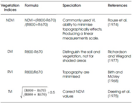
Table 2. Characteristics and Formula of Four Main Vegetation Indices used in the Study
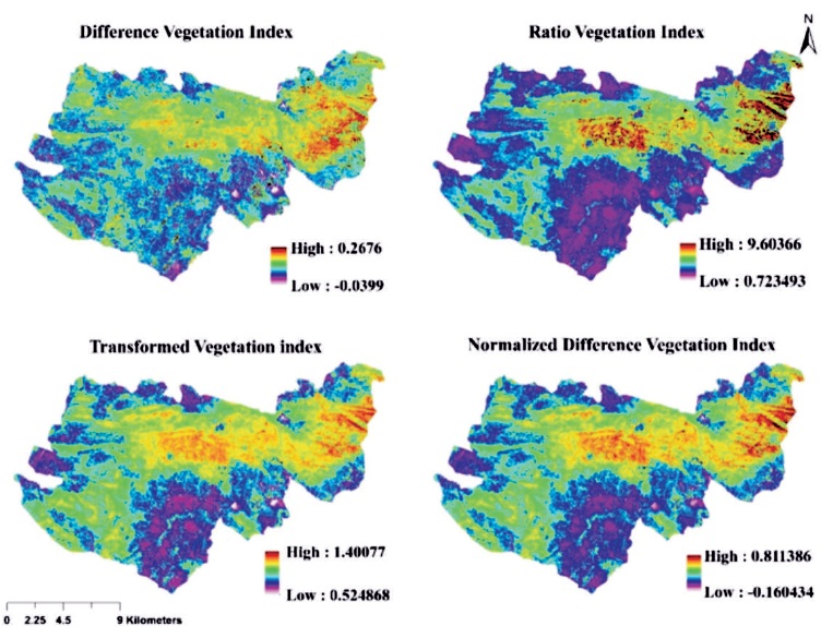
Figure 3. Vegetation Indices
The SNAP (Sentinel Application Platform) is right now accessible and is customized for the synchronous utilization of information gained by Sentinel-1, Sentinel-2, and Sentinel-3 satellites (Addabbo et al., 2016). The SNAP software was utilized to handle the Fraction of Vegetation Cover (FVC) from its biophysical processor given in its optical tool box. For the calculation of FVC, the software firstly converts the bands into the Top of Canopy reflectance (TOC) and then it is normalized by using neural network algorithms. The FVC in the investigation is ascertained by this procedure and rescaled to 1 to 100% to get a percentage of the vegetation cover (PVC).
The concept of forest canopy density was discussed in the FCD model, which helps in evaluating forest canopy density (1 to 100%). The FCD model uses indices like Advanced Vegetation Index (AVI) sensitive to the planet's amount and vigor, Bare Soil Index (BSI) which differentiate soil from the forest canopy and Shadow index indicates the shadow caused by vegetation (Rikimaru et al., 2002; Rikimaru, 1997) (Table 3). The pre-processed images were firstly normalized to value 1 and 0. Then, using the help of raster calculator in QGIS, the indices were calculated. The Canopy Density (CD) of the forest was calculated by synthesizing the AVI, BI, and SI with the help of principal component analysis and using the FCD model (Figure 2). Then, the Canopy Density (CD) was calculated. The forest area classification was based on FCD model. The above 70% of the CD indicates dense forest, 70 to 40% indicate moderately dense forest and less than 40% is open forest.
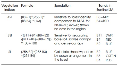
Table 3. Characteristics and Formula of Spectral Indices used for Calculating Canopy Density from Sentinel 2 A Satellite Imagery (based on FCD Model (Rikimaru, 1997))
K-Means is one of the simplest methods for analyzing, remote sensing images done by some software like Envi and Eardas Imagine (Lv et al., 2010). The process of K-means follows a simple step to categorize the given set of information to a certain number (assume k clusters) (Hartigan & Wong, 1979).
The calculated RVI, DVI, NDVI, and TVI along with PVC and canopy density was together implemented into the k-means algorithms by using SAGA GIS software. The 15 clusters were generated (Figure 4a) which consists of all the input indices and calculated PVC and canopy density. The forest classes were detected according to canopy density along with PVC. The process helps in getting separated values of vegetation indices arranged in particular cluster ID having a distinct PVC and canopy density (Table 4).
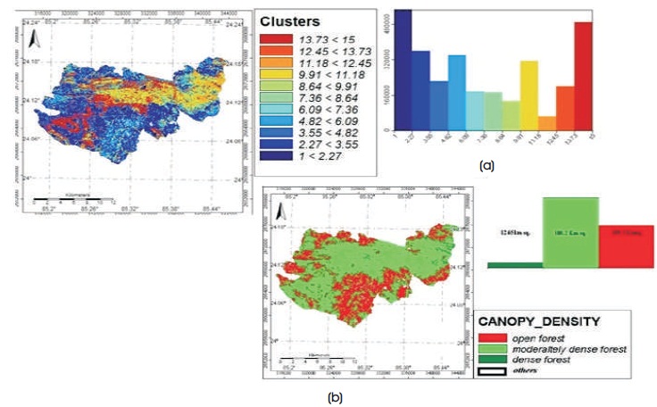
Figure 4. (a) K Mean Classification for 15 Clusters in the Study Area and its Area Frequency (b) Forest Classes based on Canopy Density
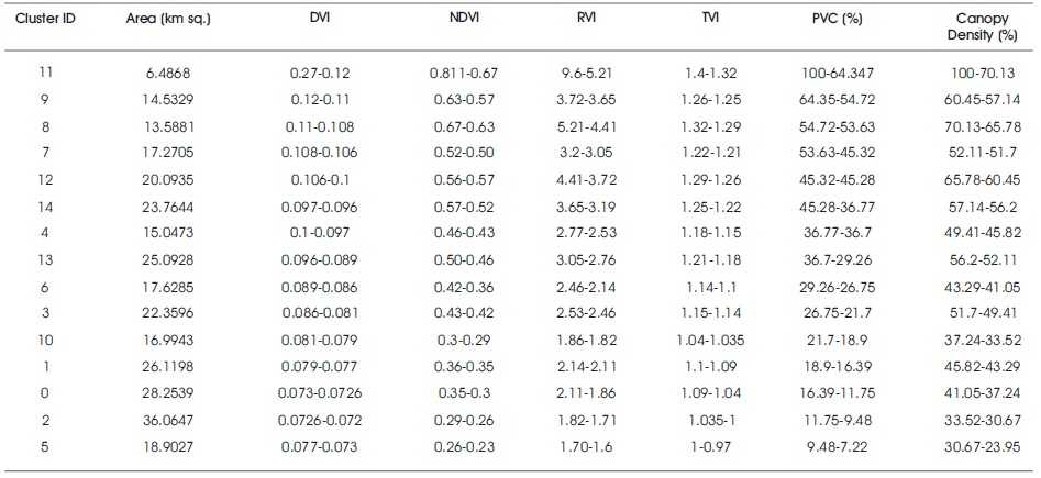
Table 4. Combined Classification of Vegetation Indices with PVC and Canopy Density
The quantification of raster values is based on the content in any imagery or raster. The quantification in other means thresholding if retrieved systematically classified into (1) interactive, (2) statistical, and (3) supervised. In the current approach, thresholds were interactively determined by visual test in cluster ID and the unsupervised approach which was based on a training set of data is used presently in K-means module.
Formation Canopy gap is a common phenomenon in a tropical forest, a normal disturbance in many forests associated with the restructuring of the forest and its community (Ostertag, 1998). In this study a canopy gap model prepared in consideration of the area other than vegetation cover are called gaps. The model predicts the percentage probability and canopy gap density (Gaps per unit area) by using calculated vegetation cover and canopy density. From the earlier study of the existing FCD model, it is clear that it is helpful in detecting canopy gaps also.
Percent probability of finding canopy gaps in vegetation cover:
P (Canopy gaps) = (100 – PVC)
Finding of canopy gap density using canopy density:
Canopy Gap Density (CGD): CGD = (100 – Canopy Density)
The first application of the current analysis was to obtain vegetation indices (Figure 3), which was further used in the context to quantify its values with canopy density PVC. For the sake of convenience and not to make complication with several results, only four vegetation indices (RVI, NDVI, DVI, and TVI) were used (Figure 3). The quantified values can also represent forest classes (Table 4b) as dense forest was having high values of VI and non-forest having low values of the VI. Forest classes are determined by canopy density based classification scheme of the forest (Forest survey of India, Dehradun).
Figure 5 contains 15 classes representing cluster Id of the quantified raster of vegetation indices, PVC, and canopy density in each ID. In this study, these classes were clustered using k-means algorithm, which is a straightforward and effective algorithm for finding clusters in data. The classification results using adjustable values of input rasters automatically come together in each cluster ID (Table 4). This analysis is possible with the help of SAGA GIS (Conrad et al., 2015).
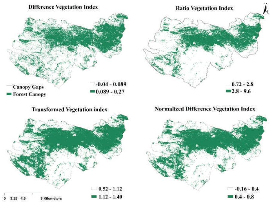
Figure 5. Potential of Vegetation Indices used for Forest Canopy Gap Detection
From the observation of clustering of 15 generated clusters (Table 4), the values of vegetation indices were picked up from the IDs and its threshold was determined (Table 5). The techniques also imply in the detection of forest classes (dense forest, moderately dense forest, and open forest) (Figure 4b) help in thresholding the values of vegetation indices that come under these forest classes (Table 5). These values of indices which was arranged by forest classes are used for finding the potential of the vegetation indices (RVI, NDVI, DVI, and TVI) for canopy gap detection (Figure 5). It is also used in mapping canopy gap probability in the forest (Figure 6).
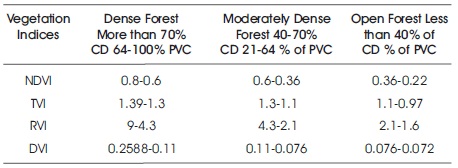
Table 5. Vegetation Indices Values Ranges for Forest Classes, Canopy Density and PVC
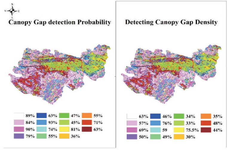
Figure 6. Probability of Finding Canopy Gaps using PVC and Clustering with K-Means
Table 5 indicates the vegetation indices values according to forest classes, vegetation indices, and PVC. The K-means clustering was helpful in thresholding the vegetation indices for dense forest, moderately dense forest, and open forest region of the study area. It was also found that dense forest (12.65 km2) having 64-100% of PVC; moderately dense forest (180.2 km2) having 21 - 64% of PVC, and open forest (109.3 km2) contains 7- 21% of PVC. The quantification of vegetation indices only contain the vegetative part of the forest (not include no-forest), where the process is only useful for monitoring plant vigor in the forest.
From the above analysis, it was found that the canopy gaps having a minimum size of 10*10 m can be defined by thresholding vegetation indices that characterized a no vegetation cover in the forest, but it is not possible to predict gap by this method as dense forest having 64-100% of PVC also contain gaps (Figure 6).
The natural (Jenks) based classification in Arc GIS separated some of the big canopy gaps in the forest (Figure 5), used for the prediction of canopy gaps and it is compared it to K-means cluster observed gaps (Figure 6). Both methods were compared and a good relationship is exhibited among them. It was found that DVI is more efficient in finding the canopy gap region, which have no vegetation, compared to other vegetation indices used. Figure 6 shows the probability of finding canopy gaps and detecting canopy gap density.
In conclusion, forest areas are complicated in nature and are full of uncertainties, which is challenging to quantify vegetation indices into different classes containing forest information. Often ground truth data are required for their accuracy estimates and hardwork is needed for their proper implications. The cluster analysis is generally faced with the problem of ground truthing to improve further accuracy. However, the research was setup after some field work and knowledge of current situations in forest. The result that calculated was observed satisfactory. The NDVI and TVI considered being more efficient and DVI was less efficient for vegetation cover and canopy density measurement. The main and unique contribution of this study was to show that range of index value for the prediction of PVC and forest classes. Further, using it the forest gaps were detected and its probability of finding was identified. Inversely, it was observed that DVI was more efficient in finding gaps in forest rather than PVC and CD, compared to slope based indices. This research also verified the utility of k-means clustering application and data transformation technique as a tool for forest landscape assessment using vegetation indices. The methodology described here can be used for a wide range of application in forests.
I would like to thank Van Bhavan, Hazaribagh Jharkhand, India for their help during field visits, RGNF for giving me a scholarship, and the Central University of Jharkhand, where I am doing Ph.D.