
This paper describes the artificial neural network application to short term load forecasting of an electrical utility. Load forecasting plays an important role in power system operation, planning and control. It has long been recognized that accurate short term load forecast represents a great savings potential for electric utility corporations. Various approaches like time series, regression, expert systems and artificial neural networks have been envisaged in power system operation. A case study using ANN based load forecasting was developed. The capability of Back Propagation algorithm and Kohonen Network have been applied for load forecasting. The performance of the above two methods is tested with the data obtained from Tamilnadu Electricity Board. The design procedure are demonstrated and sample results are presented.
Load forecasting is one of the central functions in power systems operations. The motivation for accurate forecasts lies in the nature of electricity as a commodity and trading article; electricity cannot be stored, which means that for an electric utility, the estimate of the future demand is necessary in managing the production and purchasing in an economically reasonable way. In India, the electricity markets have been recently opened, which are increasing the competition in the field . Forecasts of hourly loads for up to one week ahead are necessary for scheduling functions such as Hydro Thermal Coordination and Transaction Evaluation and for short-term analysis functions such as Dispatcher Power Flow and Optimal Power Flow. [1].
Load Forecasting in power systems can normally be broken into the following categories:
1. Very short forecasting of upto a few minutes ahead;
1. Forecasting for a lead time of upto a few days ahead;
2. Forecasting over a period from six months to one year period;
3. Long-term forecasting of power system peak load up to 10 years ahead [7].
This paper concentrates on short-term forecasting, where the prediction time varies between a few hours and about one week.
Short term load forecasting (STLF) has been lately a very commonly addressed problem in power systems literature. The methodologies typically use algorithms taken from the statistical domain or recently applied technologies from Artificial Intelligence procedure.
Traditional algorithmic techniques such as Time series and Regression approach have been reviewed briefly here.
It is based on understanding that a load pattern is nothing more than a time series signal with known seasonal, weekly, and daily periodicity. This periodicity gives a rough prediction of the load at a given time of the day. The time series approach uses a large number of complex relationships, requiring a long computational time and may result in a possible numerical instability [7].
The general procedure or the regression approach is to select the proper input variables, assume basic functional elements and find proper coefficients for the basic functional elements. This method is also characterized by long mathematical and computational procedures. The predictions were not so accurate.
The advantages of ANN over statistical models lie in its ability to model a multivariate problem without making complex dependency assumptions among input variables. Furthermore, the ANN extracts the implicit nonlinear relationship among input variables by learning from training data. These ANN extracts provide better results when compared to existing methods.
An artificial neural network is an information processing system that has certain performance characteristics similar to biological neural networks. They are elements capable of parallel processing as in human brain. A large number of models on neuro-processing have been developed, each with a variation on parallel and distributed processing ideas.
Processing elements in ANN, also known as neurons are interconnected by means of information channels called weights. Each neuron can have multiple inputs; while there can be one output. Inputs to a neuron could be from external stimuli or could be from output of other neurons. Copies of the single output that comes from a neuron could be input to many other neurons in the network.
When the weighted sum of the inputs to the neuron exceeds a certain threshold, a neuron is fired and an output signal is produced. The network can recognize input patterns once the weights are adjusted or tuned via some kind of learning process [2].
Back propagation, also known as generalized delta rule is a systematic method of training multiplayer artificial neural networks. It is built on high mathematical foundation and has a very good application potential. Even though it has its own limitations, it is applied to a wide range of practical problems and has successfully demonstrated its power [3]. In BPN, the objective of training is to adjust the weights, so that application of inputs produces the desired set of outputs. Training assumes that each input vector is paired up with a target vector representing the desired output; together these are called training pairs. Group of training pairs is called a training set [3].
The neurons in the input layer pass the input vector to the neurons in the hidden layer. The weight vectors present in between the input and hidden layers multiplies the input vector. This product is acted upon by the activation function to have the output from the hidden layer [3].
The difference between the target vector and output vector is calculated as error and based on this error value the adjustments to the weights between the hidden layer and output layer are computed. A similar correction is also made for the weights between the input and hidden layers. One presentation of each training pattern to the network is called an epoch. The epochs are increased until the error is within a prescribed tolerance [3].
In Kohonen's self-organizing feature maps, a network differentiates into multiple regions, each responsive to a specific stimulus pattern or feature. If a specific input pattern requires a specific processing function, then this self-organizing heuristic may lead to a network with functionally different regions (sub networks) [4].
The self organizing neural networks, called topology preserving maps, assume a topological structure among the cluster units. This property is observed in the brain, but is not found in other artificial neural networks. There are m cluster units, arranged in a one- or two- dimensional array [4].
The weight vector for a cluster unit serves as an example of the input patterns associated with that cluster. During the self-organization process, the cluster unit whose weight vector matches the input pattern most closely (typically, the square of the minimum Euclidean distance) is chosen as the winner. The winning unit and its neighboring unit (in terms of topology of the cluster units) update their weights. For a linear array of cluster units, the neighborhood of radius R around cluster unit J consists of all units j such that max (1, J R) j min (J + R, m) [4].
The architecture and algorithm that follows the net can be used to cluster a set of p continuous valued vectors x = (x ,……….. x…………. x ) into m clusters. The various functionalities of Kohonen network are clustering and learning.
Clustering is concerned with grouping of objects according to their similarity. In Kohonen network, clustering is done by competitive learning mechanism. Here the node with the largest activation level is declared the winner in competition. Only this node will generate an output signal and all other nodes are suppressed to the zero activation level [4].
The winning node and its neighbors will learn by adjusting their weight vectors according to the following rule

X - input vector
? - learning rate
As learning proceeds, the size of the neighborhood is gradually decreased. As the iterations increase, the number of nodes that learn decreases and finally only the winning node learns.
Two different architectures of neural networks are considered for load forecasting Back Propagation Network (BPN) and Kohonen Network. The performance of BPN is studied by changing the various network parameters like learning rate, momentum constant, epochs, numbers of hidden neurons and the activation functions. In Kohonen network also the parameters like learning rate and the epochs are changed [5]. For each model the results are obtained, error is calculated and a comparative study is made.
Data used for Training: Load profile and frequency data for 3 years from 01 Jan 2003 to 31 Dec 2005.
Data used for Testing: Load profile and frequency data for 2 months from 01 Jan 2005 to 25 Mar 2005.
All the load and frequency data are at an interval of one hour. They are obtained from Main Load Despatch Centre, Tamilnadu State Electricity Board.
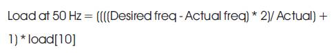
As the load data are taken in real time, the values are not at 50Hz, but at various random frequency values generally in the range of 49 to 51 Hz. This random frequency depends on the frequency of the generator which varies according to the load fluctuations. So as a first step, this load is to be corrected (standardized) for 50 Hz. The standard formula given by TNEB for this frequency correction is
As the network will accept the inputs only in the range of 1 to +1, the load data is to be linearly scaled. The general formula applied for this linear scaling is
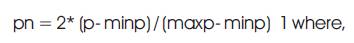
pn = linearly scaled load value
p = raw load value (MW)
maxp = maximum load value for that particular day (MW)
minp = minimum load value for that particular day (MW)
This linearly scaled load value is used for training the network. During the training phase, initially we classified the data to be trained in different groups like week days, week ends, holidays, etc, but as the results were not accurate, the raw data as such is used, without any groupings for training the network.
The network is trained i.e. the weights are updated till the stopping criteria is met. Stopping criteria can consist of a maximum number of epochs, a minimum error gradient, an error goal, etc. The trained network is tested for its performance. The load values obtained are in the range of 1 to +1[4]. So they are to be post processed to have the actual load values in MW. This is done by a post processing function given by

p = forecasted load (MW)
pn = linearly scaled load value
maxp = maximum load value for that particular day (MW)
minp = minimum load value for that particular day (MW)
In general, the overall load of Tamilnadu grows by around 6.8 % per annum due to seasonal factors and new service connections provided. But this annual load growth may not be the same all through the year [10].
The electrification of agricultural sectors is greatly influenced by the conditions peculiar to this sector, such as the subsoil water areas involved, intensity of crops, seasonal variations, etc. A large amount of electric power is consumed by electric rail road’s. At present most of the main railway lines of prime importance are electrified. Planned conversion to electric traction allows a considerable increase in the traction load. Commercial and residential usage of electric energy is growing at an ever-increasing rate. The wide use of household appliances has resulted in a growing consumption of electric energy. The demand for the domestic sector is rising very fast due to changes in life styles [1].
So in this system of load prediction, the annual load growth is calculated by considering the above-mentioned factors. Once the training and testing of the system is over, it is ready for load prediction. The system can predict the load for any day of the year 2005 and for 2006.
The performance of BPN can be improved with variations in network parameters. A proper selection of network parameter such as momentum factor, learning rate, number of hidden neurons, training algorithms are required for efficient learning and designing of a stable network.
Learning rate coefficient determines the size of weight adjustments made at each iteration and hence influences the rate of convergence. So, poor choice of coefficients can result in failure of convergence. If the learning rate coefficient is too large, the search path will oscillate and converges more slowly than a direct descent. If the coefficient is too small, descent will progress in small steps significantly increasing the time to converge. As shown in table 1, the error is minimum when the learning rate is maintained at an optimum value of 0.47.
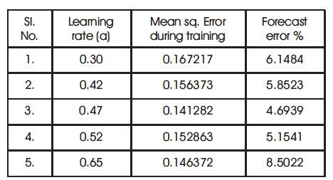
Table 1. Performance of BPN with variations in Learning Rate.
The rate of convergence can be improved by adding momentum to the gradient expression. This can be accomplished by adding a fraction of the previous weight change to the current weight change. This addition of such a term helps smooth out the descent path by preventing extreme changes in the gradients. If momentum constant is zero, the smoothening is minimal and entire weight adjustment comes from the newly calculated change. If momentum factor is one, the new adjustment is ignored and previous reading is repeated. So an optimum value between zero and one should be used to have efficient performance. In this system, a momentum constant of 0.93 gives better results (refer table 2).
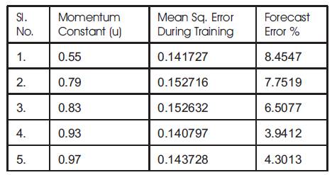
Table 2. Performance of BPN with variations in Momentum Constant
The criterion is to select the minimum nodes, which would not affect the network performance so that memory demand for storing the weights can also be kept minimum. When the number of hidden nodes is equal to the number of training patterns, the learning could be fastest. In such cases BPN loses the generalization capabilities. Hence as far as generalization is concerned, the number of hidden nodes should be small compared to number of training patterns approximately in the ratio of 10:1. Table 3 indicates that the error is minimal when 40 hidden neurons are used.
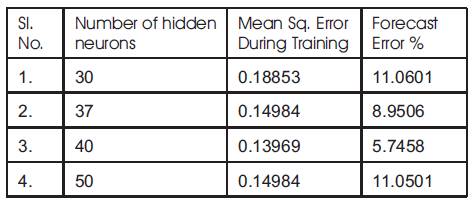
Table 3. Performance of BPN with variations in number of hidden neurons
When the network is trained for one year, the various tuning parameters that give the best results are
| Number of hidden layers | : 1 |
| Bias connect | : [1, 1] |
| Learning rate | : 0.47 |
| Momentum constant | : 0.93 |
| Number of hidden nodes | : 40 |
| Training algorithm | : trainrp |
| Activation function | :tansig, purelin |
With these above parameters, when the network was trained for two years (01 JAN 2004 to 31 DEC 2005), the forecast error was still reduced which means increase in performance (refer table 4).
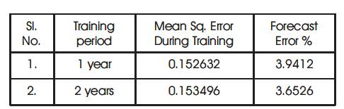
Table 4. Performance of BPN with variations in Training Period
As in the fig 1, the graph showing the performance of BPN has three plots.
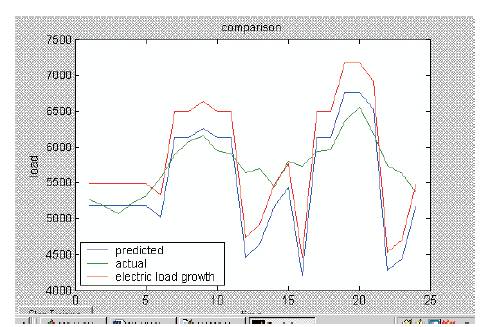
Fig 1. BPN Performance
1. The average of the actual four data (4) is fed into the network for testing.
2. The predicted load for the particular day.
3. The predicted load for the particular day considering the annual load growth.
From the graph (fig 1) it is inferred that the predicted load varies widely from the actual load, especially at two points (6 am and 2 pm) in any particular day. This is because at these points there is a shift in the load pattern.
Fig 2 depicts the performance of Kohonen network. It is inferred that the deviation of the predicted load from actual load is very minimum. As the error is very minimal, Kohonen network with the above-mentioned parameters is considered as the most suitable model for STLF.
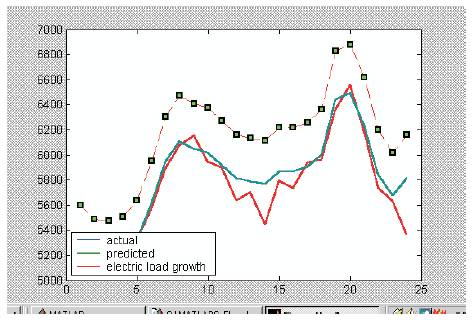
Fig 2. Kohonen Performance
Generally there occurs a change in load pattern at 6 hrs and 14 hrs of any working day. In case of BPN, the forecasted load values show abnormalities at these two points. As shown in the fig 3 the error is around 50% and because of the abnormality at these two points the average error for a BPN network works out to be 8-10%.
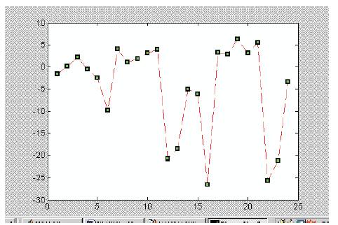
Fig 3. BPN Error Plot
In case of Kohonen network, there are no such abnormalities and the average error is around 3% (refer fig 4). Hence Kohonen network is suggested for STLF. As this new system of load prediction is more precise and accurate, the expert systems used at present in MLDC is replaced with this system and is used in real time for the load prediction.
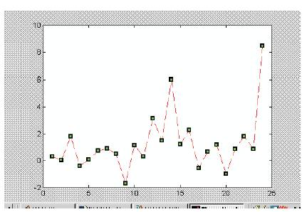
Fig 4. Kohonen Error Plot
Periodical updating (retraining) of the trained network is an important and vital aspect to be considered for the successful operation of the system. Now the network is trained with two years data (2004 & 2005) and tested with 2 months data (JAN and FEB 2005). The trained network can be used to successfully forecast the load for the entire year (2006) without requiring any updating or re-training.
But when the system is to be used for the successive years (2006, 2007,…), the network has to be retrained by the end of 2006. One possible approach is to retrain the network with cumulative load data of the available years i.e. by the end of the 2006, retrain the network with the load data of 2004, 2005 and 2006. Second possible approach is, at the end of each year always the network should be retrained using the load data of the latest two years i.e. by the end of 2006, and retrain the network with the load data of 2005 and 2006.
Electric load forecasting is an essential procedure for any energy or electric utility. Reliable operation of a power system and economical utilization of its resources require load forecasting in a wide range of time leads, from few minutes to several days. It is also useful for system security and maintenance. Though lots of conventional techniques are available, the Artificial Neural Network technique for Short Term Load Forecasting (STLF) has gained a lot of attention recently. The performance is comparatively better than the other conventional techniques.