Effect of Noise

In recent times, increasing exposure to noise pollution has become a serious problem for most of the cities. Noise affects the human health unfavorably both physically and psychologically (Serkan et al. 2008). Hospitals are the most sensitive to the exposure to noise pollution. Noise environment not only affects the patient's health but also the staff working in noisy situation. Staff find it harder to concentrate on their job, leading to them being more fatigue, with decreased performance and increased chances of error (Tsion et. al.1998). Previous investigators who studied the effects of the noise on health and healing have registered high noise levels in hospitals, showing that the problem is more serious in Intensive Care Units, both at night and during the day (Tsion et al.1998; Hilton 1985; Neriman et al 2008). The epidemic of noise in hospitals, which is one of the biggest complaints of patients and staff, is something that can no longer be ignored. Cardiac patients being the one who are adversely affected by noise during their hospital stay, they suffer from sleep disturbance, restlessness and disorientation. In addition, it also effects the elevated blood pressure, heart rate, and peripheral resistance by the release of hormones such as norepinehrine, epinephrine, and cortisol ( Tsion et. al.1998). In spite of the effort taken by the hospital and regulatory authority, the noise environment in hospital settings in India is generally an unnoticed crisis (Mackenzie et al. 2007). Very few studies are reported specially for hospitals in India on assessment of noise levels and its impacts. A serious effort is therefore needed to control the noise within the hospitals and reduce its negative impact on the patients and staff. Recent efforts are focused towards monitoring and calculating actual noise exposure and level of annoyance to the patients to actually understand the gravity of the problem due to noise in the hospital (Hilton 1985).

Sources of Noise

Noise pollution within hospital facilities are mainly caused due to equipments and machinery used during normal work activities and other human activity. The multiple monitors, beepers, buzzers, paging systems, telephones, carts, wheel chairs & gurneys, hospital beds, pillow speakers and nurses call systems, 4 poles that role on tiled floors, doors that close abruptly, and carts that squeak, all contribute to increase the noise in the hospital environment (Tsion et al.1998; Neriman et al 2008). Apart from engineering and architectural design, facilities and equipment and, of course, people are paramount (Tsion et al.1998; Hilton 1985).

Standards and Guidelines

World Health Organization (WHO) recommends noise levels limit of 40 dB (A) during the day and 35 dB (A) at nights in hospital (Tsion et al.1998; Mackenzie et al. 2007). In India, the Noise Pollution (Regulation and Control) Rules, 2000 and 2010 have been framed under the ambit of Environment (Protection) Act, 1986. The ambient levels of noise for silence zones such as hospitals is about 50 dB (A) during the day and 40 dB (A) at nights (CPCB 2000).

Noise Descriptors

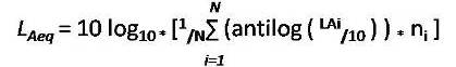
Noise is commonly used to describe sounds that are disagreeable or unpleasant produced by acoustic waves of random intensities and frequencies or without musical quality, disrupts performance, or sound that causes subjective annoyance and irritation, and it is an obnoxious stimulus for people ( Narendra et.al.2004 ) . Equivalentnoise level (LAeq) is the commonly used index which indicates that an equivalent noise would generate the same magnitude or quantum of energy as those of all readings over the given duration, covering all fluctuations. Noise Pollution Level (LNP) is another index which is used for analysis that takes into account of the variations in the sound signal and hence it should serve as a better indicator of pollution in the environment for both physical and psychological disturbances of people (Tsion et al.1998 ; Ayr et al. 2003 ; Gulab 2006). Following are the expressions used for the analysis in this present study:

(1)

(2)

(3)

Noise Pollution Level

(4)

Study Area

A premier 100 bedded cardiac hospital with all modern facilities in cardiology located at Nagpur, India is selected for the present case study. It has a cardiac operation theater that matches world standard of A-bacterial environment with the use of Module Laminar Air Flow System. Cardiac interventional procedures which include Coronary Angiographies, Coronary Angioplasties, Balloon Mitral Valvuloplasties, Pacemaker Implantations, Open and Closed Heart Surgeries are normally performed in this hospital. On an average 9 to 10 number of Heart surgeries are performed every day in that hospital and over 90 % of indoor facility of the hospital is normally booked throughout the year. A 14 Bedded ICU and 35 bedded post operative wards are available in this hospital. The Out Patient Department (OPD) is in the morning hours 9.30 - 11.30 hrs and about 80 to 90 OPD patients visited the hospital every day. Equal number of floating population (eg: patient's relatives) visit the hospital in the morning hours (9.30 -11.30 hrs) and in the evening (17:00 to 19:00 hrs).

All measurements are made through Precision-grade Sound Level Meter DAWE (Model No. 1421C), with the measuring height fixed about 1.5 m above ground surface. This measuring device is calibrated every time before use. The instrument is held comfortably, with the microphone pointed at the suspected noise source at a distance not less than 1 m away from the reflecting object. This takes care to minimize all type of error during measurement. The locations for measurements of sound level identified in hospital include reception cum registration counter, ward corridors, general ward, waiting area, outpatient department, Nursing station and intensive care unit. The criteria for selection is based on the exposure characteristics of the study area, physical characteristics of all the sampling locations and population characteristics which gives true representative of the sampled population of the complete hospital area. Measurements are recorded on a daily basis for the 16 hrs duration for the four different duration of the day (i.e. morning 6:00–11:00 a.m., afternoon 11:00–4:00 p.m., evening 4:00–7:00 p.m., and night 7:00–10:00 p.m.) with time intervals of 30 minutes at all selected sampling locations. From all the measurements of the duration, various indices are computed for analysis.

2.1 Noise Measurement

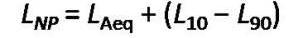
The variations in Sound Pressure Level (SPL) measured at various sampling stations are shown in Figure 1 which indicate large fluctuation in sound pressure level (SPL) in general ward, ranges from 50-85 dB(A) throughout the measurement period. The highest peak of sound pressure level is recorded, when the cleaning operation is carried out in the general ward during the meal time. The lowest SPL is observed in the night. The observed value of SPL ranges from 50- 68 dB(A) within the intensive care unit. The plot reveals that the reception and ward corridor has the highest noise levels, followed by outpatient department and waiting area, due to high population density, talking, mobile, children playing, and general activity carried by patients, patient's family member, and visitors.

To understand the percentage of time the noise level exceeded a particular value as plotted in Figure 2. It reveals that, the noise level limit of 50 dB(A) is always exceeded over the entire measurement period. On comparing the selected location, it is observed that noise level of 66 dB(A) to 69 dB(A) remained during most part of time of measurement period at reception and out patients department, Where as noise level of 58 dB(A) to 60 dB(A) exceeds 50 % of time of measurement period at general ward and intensive care unit. A noise level of 75 dB(A) exceeded 6.03 % of times during the entire measurement period at the reception. The maximum recorded sound pressure level at any time is 85 dB(A) at the general ward during the cleaning process.

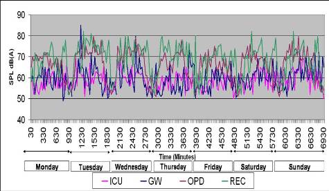
Figure 1. Plot shows SPL variation over measurement period at various sampling stations of Cardiac Hospital

Figure 2. Plot shows % Exceeding Noise Level over measurement period at various sampling stations of Cardiac Hospital.

Influence of the characteristics of the locations and period of the day on Equivalent Noise Level (LAeq) and Noise Pollution Level (LNP) are studied. There is variation in the noise exposure levels with the period of the day and the nature of the location. Figures 3 and 4 show variations of equivalent noise levels and noise pollution level with location and period of the day. The observed equivalent noise level was generally high during the daytime (6:00 am – 4:00 pm) compared with the nighttime (4:00 pm–10:00 pm). Characteristics of the location and presence of intrusive noise sources are the major factors found to be responsible for differences in noise level in the different sampling location analysed. At all sampling locations both the ( LNP) and (LAeq) rises from morning and reach peak values in the afternoon and evening but descend in the night to lower levels. The high noise exposure levels in the morning and evening at those locations can be justified as a result of morning rushing hours of patients, staff, visitors and due to conversation and discussion among the patients, staff and nurses. The noise pollution levels in the evening time (4:00 pm–7:00 pm) at intensive care unit and out patient's department areas are generally low. This is because the majority of the staff nurses were not available. Therefore population density is low at this time.

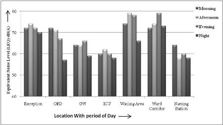
Figure 3. Variation of the Equivalent Noise Levels (Laeq) with location and period of the day

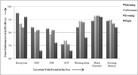
Figure 4. Variation of the Noise Pollution Levels (LNP) with location and period of the day

At the time of measurement the noise equivalent level range from 53 dB(A) to 77 dB(A). In the general ward and intensive care unit the equivalent noise levels (LAeq) value are observed as 64 dB(A) and 60 dB(A) due to doctor's round and discussion among the patients with their relatives. The highest and lowest noise pollution level (LNP) are observed as 95 dB(A) and 66 dB(A) respectively. The higher noise pollution level (LNP) during the morning period is 95 dB(A) at reception and 84 dB(A) at outpatients department is obtained when loud conversation and pulling of chairs is found to be a causative factor at that moment. The higher noise pollution level (LNP) during the morning period of 83 dB(A) and 71 dB(A) is obtained in general ward and intensive care unit respectively, and changing of beds and beeping noise generated by equipment at intensive care unit is found to the source at that moment. Reception and out patients department are found to be the noisiest sites with peak noise levels (L10) of 79 dB(A) and 72 dB(A), respectively, compared to the peak noise value at general ward and intensive care unit of 72 dB(A) and 67 dB(A) respectively. The highest noise level is produced by snoring, crying in pain of surrounding patients in general ward and intensive care unit. But at reception and out patients department, the high noise levels may be a result of the noise produced by various activity carried by patients and their relatives or visitors. The use of electronic appliances such as radio, mobile and printer at the reception and out patients department is become the main causative factor for creating substantial amount of noise level. Noise from nearby surrounding commercial activities and the traffic noise are another sources contributing to the environmental noise. The (L90) value shows the noise level between 52.75 dB(A) to 53.25 dB(A) occurs due to the normal work activity and normal conversation. This commensurate with the obser vation made for environmental sound levels with number of specific variables determining the characteristics and sources of noise present at the location(Ahmed et al. 2006; Olayinka et al. 2010).

In order to determine whether there is difference in noise exposure level at all the sampling locations, they are surveyed throughout the measurement period (i.e. from morning to night) to find if they are significant or not. The data is analyzed through ANOVA (Analysis of Variance) for single factor experiment, using F- distribution which is carried out on equivalent noise level (LAeq) and noise pollution level (LNP). Table 1 and Table 2 show the analysis of variance tables for noise equivalent levels (LAeq), and noise pollution levels (LNP) respectively. At 95% confidence level, the Mean Square Ratio (MSR) calculated for equivalent noise level (LAeq) is 10.07, while the tabulated value is 2.57 (Lipson et al. 1973). Similarly, at the same confidence level, the (MSR) calculated for noise pollution level (LNP) is 9.01 and the tabulated value remains as 2.57. Since, in both the cases, the calculated (MSR) is greater than the tabulated value, there is a significant difference (p< 0.05) in the equivalent noise level (LAeq) and noise pollution level (LNP) in the locations surveyed based on the data analyzed at 95% confidence level.

2.2 Noise Prediction Model

The time series of noise level obtained as a result of sampling of instantaneous noise measured in the hospital environment is analyzed using ARIMA technique (Kumar et al. 1999). A general ARIMA model of order (p,d,q) representing the time series can be written as

 

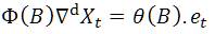
Where x_t and e_t represent sound pressure level and  random error terms at time (t) respectively. B is a backward shift operator defined by B x_t = x_t -1, and related to 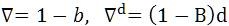, d is the order of differencing. Φ (B) and θ (B) are Auto Regressive (AR) and Moving Averages (MA) operators of orders p and q, respectively, and are defined as given by,

(4)

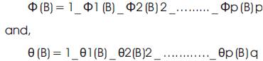
Where Φ1, Φ2… Φp are the auto regressive coefficients and θ1, θ2 … θp are the moving average coefficients.

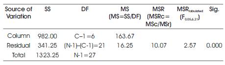
Table 1. Analysis of variance for equivalent noise level (Laeq)

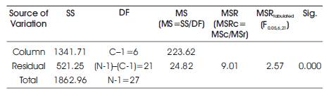
Table 2. Analysis of variance for noise pollution level (LNP)

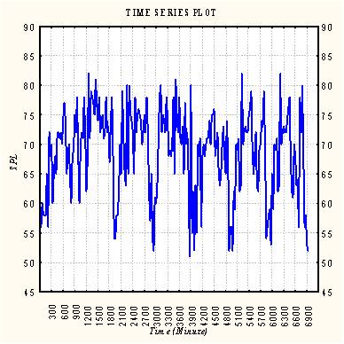
Figure 5. Time sequence plot

In the Box-Jenkins Methodology of ARIMA modeling, the first step is to determine whether the time series is stationary or non stationary. If it is non-stationary it is transformed into a stationary time series by applying suitable degree of differencing to it. This gives the value of d. Then appropriate values of p and q are found by examining Auto Correlation Function (ACF) and Partial Auto-correlation Function (PACF) of the time series. Having determined p and q and d the coefficients of autoregressive and moving average terms are estimated using nonlinear least squares method (Box et al. 1976). In the present study the time series has been analyzed using statistical computer software (STATISTICA).

Figure 5 shows the horizontal time sequence plot of the time series of noise levels. The time series appears to be stationary as far as its non-seasonal behavior is concerned. In the Box-Jenkins methodology of ARIMA modeling, it must be first established that the given time series is stationary before trying to identify the orders of AR and MA processes in the model to be fitted. The ACF of a time series is an important tool in this regard.

Figure 6 shows the ACF of time series of noise levels obtained in the present study. It can be clearly seen that the auto correlations are significantly different from zero even at higher time lags. It may be also noticed that the auto correlations form a wave-like pattern. If one combines the behaviors indicated by Figures 5 and 6, it can be inferred that the time series may have some seasonal non-stationarity. A more careful examination of Figure 6 reveals that the autocorrelations at lags 15, 30 are unusually high. The neighboring autocorrelations at lags 14, 29,... are also on the higher sides. This indicates that the presence of seasonality (roughly of the length 15) in the given time series, may be associated with the visitor present at the reception.

This can be confirmed by the seasonal subseries plot (season length=15) of the time series shown in Figure 7. It is evident from the figure that, the seasonal means are not same for all the 15 seasons. Instead, a wave-like pattern is observed in seasonal means. Figures 5 and 7 therefore point towards the presence of a seasonal non-stationarity of about the length 15 in the given time series. In view of the indications, it becomes desirable to do the seasonal differencing of the original time series in order to remove the existing seasonal non stationarity. Thus, a new time series is generated by differencing the original time series at lag 15.

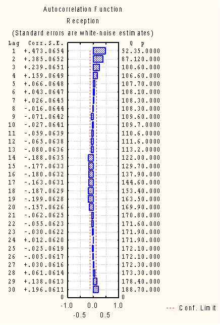
Figure 6. ACF of Time series

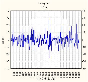
Figure 7. Seasonal sub series plot

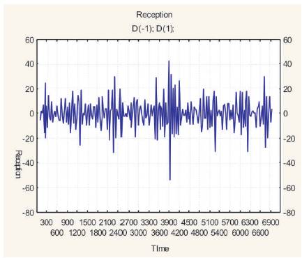
Figure 8. Seasonal sub-series plot of the seasonally differenced time series

Figure 8 shows the seasonal subseries plot of this new time series. It becomes clear at once that the seasonal means are almost the same for all seasons now. In other words, the seasonal non stationarity appears to have been removed in this new time series.

Figure 9 shows the ACF of this differenced time series. It can be seen that the autocorrelation at lag 15 is significantly different from zero. All the other autocorrelations may be considered as insignificant. Figure 9 shows the PACF of the seasonally differenced series. It can be observed that there is a pattern of exponential decay in the partial autocorrelations at lag 15, 30, ... The patterns observed in Figures 9 and 10 are quite similar to the theoretical patterns of ACF and PACF of a seasonal MA process of the order 1. This indicates that the existence of a seasonal MA process of order 1 in the original time series. In view of the observations a seasonal model of the order (0,1,1) [15] was identified. Here p =0, q =1, d =1 and the superscript 15 represents the length of seasonality. The model fitting results are given in Table 3.

It can be seen from the table that the value of the seasonal moving average parameter θ₁ is less than 1  which confirms the condition of invertibility required for moving average coefficients. Further, the p-value obtained for θ₁ is very good, thus indicating that the value  of the coefficient is significantly different from zero. The pvalue obtained for the mean indicates that cannot be taken as significantly different from zero. This is of course expected since the original time series has been a different once and the model, therefore, gives the mean for the seasonally differenced time series. The nonsignificant value of mean in the model further indicates the absence of deterministic trend in the original time series. In other words, it can be said that time series is stochastic in nature and that it lacks any deterministic component.

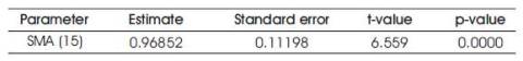
Table 3. Summary of important parameter of fitted model

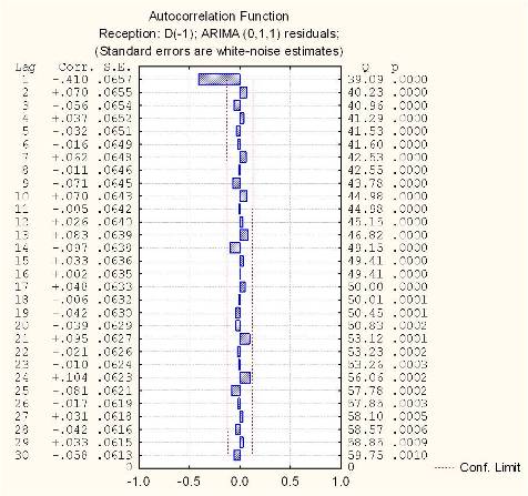
Figure 9. ACF of seasonally differenced time series

Once an ARIMA model is fitted, it is important to investigate how well the model fits the given time series. This comprises the step of diagnostic checking in model building. Investigation of the behavior of residuals is a useful tool in this regard. Figure 11 shows the ACF of residuals obtained from the model fitted in Table 3. It is evident from the figure that all autocorrelations in the ACF plot of residuals are insignificant. This implies that the residuals are not auto-correlated and are statistically independent. This means that the model is adequate. The results of observed time series of noise levels are given in Table 3. The model developed on this basis is given in Equation (5),

(5)

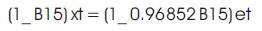
One of the basic principles of ARIMA model building is that the model should be parsimonious (i.e. the model which adequately describes the time series with a relatively less number of parameters). Keeping in view of the principle, it can be concluded that the model represented by Eq. (5) is the most appropriate for the observed time series. The model Equation (5) can be used for predictive purposes by expanding it in the following manner.

(6)

Where, t is assumed to be the current time period (i.e. the 231st, the last observation).

In order to forecast x_t+1, all the subscripts in Eq. (5) are increased by 1 which is given by,

(7)

Since the term e_t+1 that is the forecast error one period ahead is not known, it is assigned the value of zero (the expected value of feature random errors). The values of other terms on the right-hand side of Equation (7) are known. Thus the forecast one period ahead is determined. Forecasts for future periods can similarly be obtained. To summarize, the road traffic noise variations in this present study have been shown to be governed by a seasonal moving average (0,1,1) process. It would be appropriate to mention that, the result cannot be generalized to other traffic sites. In fact the identification of the stochastic process (whether autoregressive or moving average or a combination of both) governing any time series will have to be done a fresh in order to develop a predictive model of noise level for a given sampling station. The utility of the time series modeling approach in the present study is limited in so much as the forecasting of long-term noise levels is concerned. However, the study reveals that, even on short time scales, the fluctuations in noise levels are governed by stochastic processes which can be identified with the help of the Box-Jenkins methodology. Certainly, it would have been better to consider a time series over much longer time scales (e.g. months or years) but it was not feasible in the present study due to the lack of the facility of a permanent automatic noise monitoring station. Nevertheless, the adequacy of ARIMA modeling technique demonstrated in the present study provides the basis to further investigate the applicability of those techniques to forecast noise levels over longer time scales.

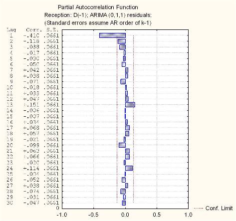
Figure 10. PACF of seasonally differenced time series

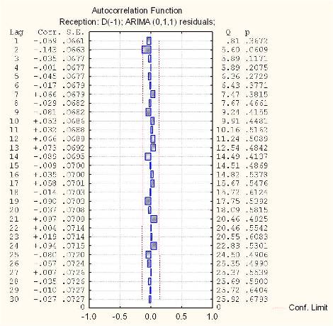
Figure 11. Estimated residual ACF

The present field study in cardiac hospital environment shows a high equivalent noise level (LAeq) ranging between 59.93 dB(A) to 72.10 dB(A) than the ambient noise level limit prescribed by any regulatory authority in sensitive areas including hospitals. A significant difference in noise exposure levels spatially and temporally (p < 0.05) at 95 % confidence level are observed at various locations including intensive care unit and wards. A high noise levels is registered during the afternoon (LAeq = 67.96 dB) and at morning (LAeq = 66.79 dB). Keeping in mind the hospitalized patient, the staff of hospital needs to be aware of noise producing activity and adopt remedial measures to reduce them within permissible limit. The staffs are needed to be aware of and sensitive to the issue. Nurses are in key positions where they can identify physical, psychological and social stresses that affect patients during their hospital stay. Staff education, planned nursing activities and proper design of intensive care unit and other units may help combat this overlooked problem. A noise prediction model developed in this study can be used to forecast the noise levels both spatially and temporally within the hospital premises.

The authors gratefully acknowledge the permission granted by the hospital authority to conduct a study and they also thankful to all the respondents (namely patients, medical staff, and patients relatives) for their kind responses to this study.

The following symbols are used in this paper:
dB(A)= decibel (A-weighted);
L_Ai = The ith A-weighted sound pressure level reading in decibels;
N = Total number of readings;
L_Aeq = A-weighted equivalent sound pressure level;
L_AeqM =Equivalent sound pressure for the morning measurement
L_AeqA = Equivalent sound pressure level for the afternoon measurement;
L_AeqE = Equivalent sound pressure level for the evening measurement;
L_AeqN =Equivalent sound pressure level for the night measurement;
L_N = Nighttime noise level;
L_D = Daytime noise level;
L₁₀ = The noise level exceeded 10% of the time. This represents peak noise level;
L₅₀ = The noise level exceeded 50% of the time. This represent mean level of noise;
L₉₀ = The noise level exceeded 90% of the time. This value considered as the background noise level;
L_NP = Noise pollution level ;