This article presents a method to predict the equilibrium composition and temperature of a reaction mixture in gas phase as found in the reaction furnace of the Claus Sulphur Recovery Unit (SRU). The proposed method is useful for process design as well as plant performance optimization. An expression for the Gibbs free energy of the system in terms of temperature is derived by using the Soave-Redlich-Kwong (SRK) equation of state. Temperature correlations for Gibbs free energy of formation of various components in the reaction mixture are obtained using standard heat capacity (Cp) temperature correlations. Initial assumption for the furnace outlet temperature is made to calculate the value for the Gibbs free energy of the system. Solver function minimizes this value by varying the composition of the outlet stream using mathematical optimization methods for non-linear systems. The outlet stream composition corresponding to this value is the equilibrium composition as the Gibbs free energy of a system reaches minimum at equilibrium. Application of Gibbs free energy minimization method using the Solver feature present in the Microsoft Excel spreadsheet program is found to predict effectively the equilibrium composition and temperature of the outlet streams of reaction mixtures in three plant case studies of Claus Sulphur Recovery Unit.
Gibbs free energy minimization method can be used to predict equilibrium compositions in reacting systems involving a large number of species. It is being increasingly preferred to the traditional mass balance method as identification of all the reactions occurring in the mixture along with their extents becomes very difficult due to the large number of species involved as cited by Y Lwin [1]. If the minimum value of Gibbs free energy of a system is predicted correctly, the composition at this value would give the equilibrium composition since Gibbs free energy of any system is minimum at equilibrium.
This minimization is carried out with the help of Solver feature present in the Microsoft Excel spreadsheet package [1]. The equilibrium temperature is estimated by carrying out an enthalpy balance across the reacting system.
The case in consideration is the Claus reaction furnace in the SRU operating on the Claus process [2]. Claus process is the most widely employed industrial process to recover elemental sulphur from gaseous hydrogen sulphide (H2S). Recovery of sulphur is necessitated because of environmental regulations on emissions for several petroleum products mainly, gasoline, kerosene and diesel [3,4]. Moreover, recovery of sulphur helps in increasing the revenue in view of the wide range of applications of elemental sulphur. Hydro treatment converts the sulphur in petroleum products into H2S. Acid gas (containing H2S) is separated from hydrotreated gases by amine treatment. Moreover, H2S bearing Sour Water coming from different other sources is stripped of its H2S in Sour Water Stripper (SWS). Both these H2S containing gases are combined as feed to the SRU.
Claus process involves oxidation of a portion of H2S in the feed gas in the Claus furnace to produce sulphur dioxide (SO2). The feed is heated to around 200°C before being fed to the Claus furnace where it reacts with air preheated to the same temperature. Oxidation of 1/3rd of the total H2S takes place at a pressure of 1-2 bar in the furnace to produce SO2. The exothermic reaction raises the temperature of the furnace to around 1200°C. The resulting gas mixture is then passed through a series of catalytic Claus reactors where elemental sulphur is formed. The sulphur obtained is condensed and extracted as product.
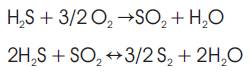
The major reactions taking place in the Claus furnace are [5].
In addition to the above, many other side reactions take place in the furnace. For example, side reactions involving hydrocarbons and CO2 present in acid gas can result in the formation of carbonyl sulphide (COS), carbon disulphide (CS2) and carbon monoxide (CO) in the furnace.
The reacting system comprises of the feed (Acid gas & SWS gas) and combustion air, at an initial temperature of about 200°C and pressure of 1-2 bar. The feed consists primarily of H2S (from Acid gas & SWS gas), N2, and O2 (from air). Besides these, H2O, CO2, and NH3 are also present along with small amounts of light paraffinic hydrocarbons (C1, C2, C3, and C4), Hydrogen and Argon. The reactions yield SO2, S2 as the main products along with CO, COS and CS2.
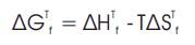
Gibbs free energy of formation (ΔGTf) of any species in the system at any temperature T is given by-
ΔHTf and, ΔSTf can be calculated using the following relations:-
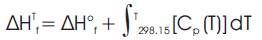
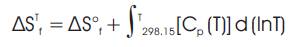
While the values for ΔH°f, standard enthalpy of formation for any species at 298.15 K, kJ/mol have been obtained directly from the available literatures, the values for ΔS°f, standard entropy of formation of any species at 298.15 K, kJ/molK had to be calculated using the following relation [6].
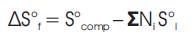
By convention, ΔH°f and ΔS°f values for elements are assumed equal to zero.
Using standard temperature dependent specific heat (Cp) correlations for different species in the reaction system, ΔGTf correlations for all species are derived using f equations (1), (2) and (3) [6,7]. These correlations are depicted in Table 1.
The total Gibbs free energy of the system is given by-
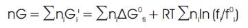
For gas phase reactions,
Since the standard state is taken as pure ideal gas state at 1 bar, f1o =1.
Substituting this we get
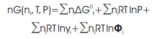
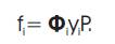
The fugacity coefficient (Φ) of each species in the mixture is calculated using the Soave-Redlich-Kwong (SRK) equation of state [8].
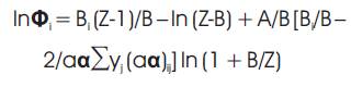
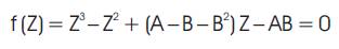
where Z is also calculated using the SRK equation of state:-
where,
Bi =bi P/RT,
B=bP/RT= (Σyi bi) P/RT,
A=aαP/ (RT)2 =(Σyi Σyj aαij)P/(RT)2,
aαij = (aαi * aαj)½ (1- kij),
ai = 0.42747R2 Tc2 /Pc
bi = 0.08664RTc /Pc,
αi = [1+m(1-(T/Tc)½ )]2 ,
m= 0.48+1.574ωi -0.176ωi2
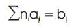
The following constraints must be satisfied for minimization of total Gibbs free energy:-
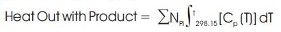
All the calculations in the preceding stages are done by assuming an outlet stream temperature [7]. Therefore, it is necessary to crosscheck this assumption. This is done by carrying out the following heat balance calculation over the Claus furnace.
Heat In with reactant – Heat Out with Product = Heat Generated (heat of Reaction) – Heat Loss

The heat generated in the reaction is the heat of reaction, which is given by the following relation:-

Thus, the correct temperature should satisfy the relation given below.

If the relation given by equation (15) is not satisfied a new value for outlet temperature is assumed and the whole process is repeated till convergence is achieved within acceptable deviation.

Table 1. ΔGTf Correlations for species in the reaction mixture
To get the correct heat balance, it is necessary to calculate the heat loss from the walls of the furnace correctly. Only heat loss due to conduction from the shell walls of the Claus furnace needs to be considered in this case [7].
The furnace is made up of three layers, first layer is the thin shell, and other two are insulating firebricks. Heat loss calculation is based on conductivity of the insulating layers, maximum shell wall temperature, wind velocity and ambient temperature (available from plant data).
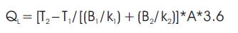
The heat loss, QL is given by the following equation:
The Gibbs free energy minimization is carried out with the help of Solver function, pre-installed in Microsoft Excel. It applies the Generalized Reduced Gradient (GRG) method to solve non-linear systems for a given set of data [1]. Typical calculation algorithm is shown in Figure 1 and Solver Parameter Dialogue Box in Figure 2.
The input data includes chemical identities of the reaction species, feed composition, furnace inlet temperature and reaction pressure. All other thermodynamic parameters namely, critical temperature, critical pressure, acentric factor, binary interaction parameter, standard heat of formation, standard Gibbs free energy of formation, absolute entropy are supplied by the user on spreadsheet based on literature data [7,9,10].
Besides these, the user has to supply the initial estimates for furnace outlet composition, outlet stream temperature, and compressibility factor, Z. The initial estimate for Z is unity.
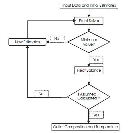
Figure 1. Algorithm for Solving the Model
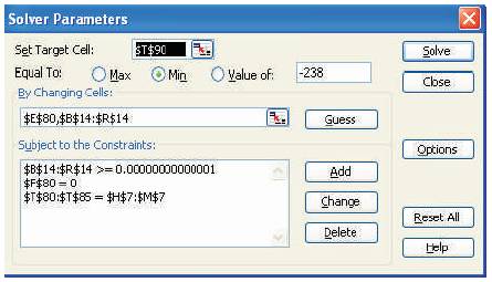
Figure 2. Solver Parameter Dialogue Box
The various equations described in the previous section are entered to calculate the necessary values using above-mentioned input data. A model spreadsheet is shown in Tables 5 (A), 5 (B) and 5 (C). To operate the Solver, the user needs to specify the objective function, the decision variables, and the constraint functions in the 'Solver Parameter' dialogue box.
After these have been defined and the Solver search conditions and parameters have been adjusted, the Solver is run by clicking on the 'Solve' button. When an optimal solution is achieved, Solver displays a message 'Solver found a solution, all constraints and optimality conditions are satisfied'. This indicates that the Solver has found a locally optimal solution. The Solver should be run from several sets of initial estimates to ensure that a globally optimal solution has been found with the minimum possible value of nG. Since Solver is a completely mathematical optimization tool, widely different sets of initial estimates may lead to different sets of solutions. Therefore, to ensure that the globally optimal solutions is obtained, it is advisable to provide initial estimates close to the optimal values and look for the solution with the lowest value of nG.
On this model spreadsheet, the total Gibbs free energy of the system (nG), given by equation (7) occupies the objective function target cell (T90) which needs to be minimized.
The outlet stream composition (moles) and the compressibility factor, Z represented by cell numbers B14 toR14 and E80 respectively, occupy the decision variable change cells.
The equation '$H$7:$M$7=$T$80:$T$85' represents elemental balance constraint on the spreadsheet.
The cells B14 to R14 must be maintained strictly greater than zero to satisfy the non-negativity constraint. This constraint tends to get violated in the GRG method used by the Solver. Thus, to keep the mole numbers strictly greater than zero so that the Solver runs without being interrupted by error messages, MAX function present in the Excel spreadsheet can be used to replace the nonnegativity constraint. For this, the cells B13 to R13 (initial estimates) should be labelled as change cells instead of B14 to R14. Simultaneously, MAX function should be used in the cells B14 to R14 so that they represent the largest value between the corresponding change cells and a small positive quantity. For example, cell B14 should be formulated as 'MAX (0.0001,B13)'.
The value of the function f(Z) given by equation (9) must be equal to zero. It is represented by cell number F80.
The results provided by the Solver for the outlet stream composition and the outlet stream temperature are compared with the plant (referred case study) furnace outlet composition at different SRU plants using corresponding feed compositions and inlet temperature. The comparison is depicted in the following tables (Tables 2- 4).
Solver calculated outlet composition with respect to key components like H2S, O2, H2O, SO2 and Sx for Plant 1 found to match reasonably well with actual plant outlet composition.
The calculated outlet temperature is for plant 1 found to be 1544 °K, whereas, the outlet temperature according to plant data is 1541 °K.
Estimated temperature for Plant 1 accounts for calculated heat loss of 365293.38 kJ/hr, which is about 2.97% of the heat of reaction.
Solver calculated outlet composition with respect to key components like H2S, O2, H2O, SO2 and Sx for Plant 2 found to match reasonably well with actual plant outlet composition.
Similarly, the calculated outlet temperature for Plant 2 is found to be 1551 °K, whereas the outlet temperature according to plant data is 1563.5 °K.
Solver calculated outlet composition with respect to key components like H2S, O2, H2O,SO2 and Sx for Plant 3 found to match reasonably well with actual plant outlet composition.
The calculated outlet temperature for Plant 3 is found to be 1540.5 °K, whereas the outlet temperature according to design data is 1546 °K.
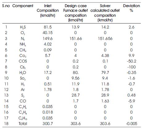
Table 2. Comparison of Solver calculated and Plant Outlet Composition (Plant 1)
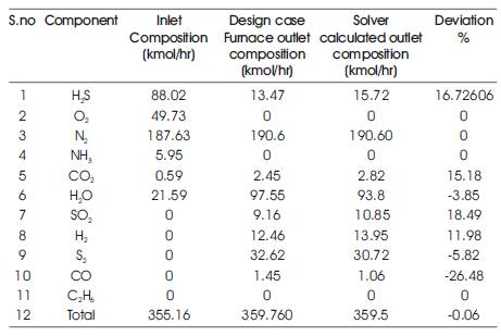
Table 3. Comparison of Solver calculated and Plant Outlet Composition (Plant 2)

Table 4. Comparison of Solver calculated and Plant Outlet Composition (Plant 3)
From the results, it is concluded that the Solver Feature in Microsoft Excel can be effectively used to predict the Claus Furnace Outlet Composition based on Gibbs Free Energy Minimization technique. The results give reasonably good prediction with respect to critical components like H2S, SO2, S2, H2O, CO2 etc for further calculation of Claus catalytic reaction steps. This in turn provides a good process-engineering basis for the Claus Reaction Furnace and Sulphur Recovery Technology covering the steam generation potential. The deviations in the predictions for non-key components (with low concentrations) like COS, CS2, NH3 and CO may be due to convergence criteria of solver correlation used to estimate the Gibbs free energy of these components. However, all above three results indicate that this tool can be used for quick prediction/evaluation of Claus Furnace design/operation with respect to key components like H2S, O2, H2OSO2, Sx and temperature.
| aji | number of gram atoms of element j in one mole of species i |
| A | surface area of the shell wall, sq.m |
| bj | number of moles of element j in the feed stream |
| B1 | thickness of the first insulating layer, m |
| B2 | thickness of the second insulating layer, m |
| Cp | specific heat capacity of any species, kJ/molK |
| f1 | fugacity of species i in the gas mixture |
| fi0 | fugacity of species i at its standard state |
| ΔGTf | Gibbs free energy of formation of any species at f temperature T, kJ/mol |
| ΔG°f | Gibbs free energy of formation of any species at f 298.15 K, kJ/mol |
| nG | Total Gibbs free energy of the system, kJ/mol |
| ΔHTf | heat of formation of any species at temperature T, f kJ/mol |
| ΔH°f | standard enthalpy of formation of any species at f 298.15 K, kJ/mol |
| ΔH°R | heat of reaction at 298.15 K, kJ/hr |
| k1 | thermal conductivity of first insulating layer, W/mK |
| k2 | thermal conductivity of second insulating layer, W/mK |
| ki | binary interaction parameter |
| ni | number of moles of species i in the outlet stream |
| Ni | number of moles of element i in one mole of the compound |
| NRi | number of moles of species i in the feed |
| NPi | number of moles of species i in the outlet |
| Pc | Critical Pressure, bar |
| QL | heat loss through the shell wall, kJ/hr |
| R | Gas constant , kJ/molK |
| S°i | absolute entropy of element i in its standard state at i 298.15 K, kJ/molK |
| S°comp | ideal gas absolute entropy of the compound at comp 298.15 K, kJ/molK |
| ΔSTf | entropy of formation of any species at temperature T, kJ/molK |
| ΔS°f | standard entropy of formation for any species at f 298.15 K, kJ/molK |
| T1 | shell wall temperature, K |
| T2 | process gas temperature, K |
| Tc | Critical Temperature, K |
| yi | mole fraction of component i. |
| Z | compressibility factor |
| Φi | fugacity coefficient of species i in the gas mixture |
| ωi | acentric factor. |
| 1. | B3 to R3 - Chemical identities of all the species namely- H2S, O2, N2, NH3, CH4, CO2, COS, CS2, H2O, SO2, H2, Ar, S2, CO, C2H6, C3H8 and C4H10, respectively. |
| 2. | B4 to R4 - Starting moles of all the species in the feed stream. S4 - Total no. of moles in feed stream. |
| 3. | B6 - Furnace flame temperature. B7- Reaction pressure. B8- Universal gas constant. B9-Product of gas constant and furnace flame temperature. D7- Acid gas inlet temperature. D8- Combustion air temperature. |
| 4. | H7 to M7- Moles of all the elements in the feed stream. |
| 5. | B12 to R12- Moles of all species in the outlet stream as per plant data. |
| 6. | 6. B13 to R13- Change cells for number of moles of all species in the outlet stream. |
| 7. | B14 to R14- Moles(n ) of all species in the outlet stream as calculated by Solver. |
| 8. | B15 to R15- Mole fractions (y ) of all species as per the i outlet stream composition calculated by Solver. |
| 9. | B16 to R16- Percentage deviations of the Solver predictions for outlet compositions from the plant data. |
| 10. | B18 to R18- Gibbs free energy of formation of all species at furnace flame temperature. |
| 11. | B19 to R19- Critical temperatures of all species. |
| 12. | B20 to R20- Critical pressures of all species. |
| 13. | B21 to R21- Acentric factors for all species |
| 14. | B22 to R22- ai values for all species |
| 15. | B23 to R23- bi values for all species. S23- b= Σyi bi |
| 16. | B24 to R24- m values for all species. |
| 17. | B25 to R25- Reduced temperatures for all species. |
| 18. | B26 to R26- Reduced pressures for all species. |
| 19. | B27 to R27- αi values for all species. |
| 20. | B28 to R28- aαi values for all species. |
| 21. | B29 to R29- Ai values for all species. |
| 22. | B30 to R30- Bi values for all species. |
| 23. | B33 to R38- Atomic matrix for each element with respect to each species. |
| 24. | B42 to R58- Binary interaction parameters for all species. |
| 25. | B61 to R77- aαij values for all species. |
| 26. | S61 to S77- Σyj aαij values for all species. T61 to T77- yi * Σyi aαij values for all species. S79- aα value for the system. |
| 27. | B80- A value for the system. C80- B value for the system. |
| 28. | B82 to R82- 'Bi (Z-1)/B – ln (Z-B)' values for all species. |
| 29. | B83 to R83- Σyj aαij values for all species. |
| 30. | E80- Z value. F80- f(Z) function to determine Z. |
| 31. | B85 to R85- logarithmic values for fugacity coefficient for all species. |
| 32. | B87 to R87- Molecular weights of all species. |
| 33. | B88 to R88- Mass of each species in the feed stream. |
| 34. | B89 to R89- Mass of each species in the outlet stream. |
| 35. | T80 to T85- Moles of all elements in the outlet stream. |
| 36. | T86 to T89- Σni ΔGTf, Σni RT lnP, Σni RT lnyi and Σni RT lnΦi values for all species. |
| 37. | T90- Total Gibbs free energy of the system. |
| 38. | T91- Ratio of moles of H2S to moles of SO2 in the outlet stream. |
| 39. | B90 to R90- Heat input to the system by each reactant species. |
| 40. | B96 toR96- Heat input to the system by one mole of each reactant species. |
| 41. | T93- Total heat input to the system by the reactants. |
| 42. | B91 to R91- Heat output from the system with each product species. |
| 43. | B100 toR100- Heat output from the system with one mole of each product species. |
| 44. | T94- Total heat output from the system with the products. |
| 45. | T95- Available sensible heat. |
| 46. | B94 to R94- Standard heat of formation of one mole of each species at 298.15 K. |
| 47. | B97 to R97- Standard heat of formation of each reactant species at 298.15 K. |
| 48. | T97- Total heat of formation of reactants at 298.15 K. |
| 49. | B99 to R99- Standard heat of formation of each product species at 298.15 K. |
| 50. | T99- Total heat of formation of products at 298.15 K. |
| 51. | T100- Heat of reaction |
| 52. | T101- Heat loss |
| 53. | T103- Net heat of reaction. |
| 54. | T104- Deviation of available sensible heat from net heat of reaction. |
| 55. | T105- Percentage of heat loss. |
| 56. | D108 to D137- Standard Gibbs free energy of formation of any species at 298.15 K, kJ/mol |
| 57. | E108 to E137- Ideal gas absolute entropy of each species at 298.15 K, kJ/molK |
| 58. | F108 to F137- Standard entropy of formation for any species at 298.15 K, kJ/molK |
| 59. | G108 to G137- Change in the entropy of each species from 298.15 K to furnace flame temperature. |
| 60. | Q109 and R109- Process gas temperature for the minimum and maximum heat loss cases respectively. |
| 61. | Q110 and R110- Ambient temperature for the minimum and maximum heat loss cases respectively. |
| 62. | Q111 and R111- Wind velocity for minimum and maximum heat loss cases respectively. |
| 63. | Q112 and R112- Shell wall temperature for minimum and maximum heat loss cases respectively. |
| 64. | M114 and P114- Thickness of insulation firebricks. |
| 65. | M115 to P119- Thermal conductivities of insulation firebricks at different temperatures. |
| 66. | M120 and P120- Average thermal conductivity of insulation firebricks. |
| 67. | K126- Outer diameter of the reaction furnace. |
| 68. | L126- Total thickness of the insulation firebricks layer. |
| 69. | M126- Inner diameter of the reaction furnace. |
| 70. | N126- Logarithmic mean diameter of the reaction furnace. |
| 71. | O126- Length of the reaction furnace. |
| 72. | P126- Surface area of the furnace wall. |
| 73. | L129 and M129- Heat loss per unit area for the minimum and maximum heat loss cases respectively. |
| 74. | O129 and P129- Total heat loss in Watts for the minimum and maximum heat loss cases respectively. |
| 75. | Q129 and R129- Total heat loss in kJ/hr for the minimum and maximum heat loss cases respectively. |
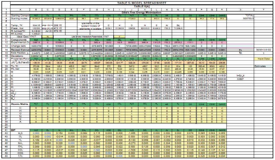
Table 5(a). Model Spreadsheet A1 to T49
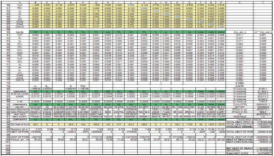
Table 5(b). Model Spreadsheet A50 to T105
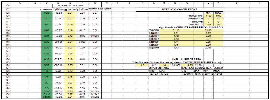
Table 5( c). Model Spreadsheet A106 to T137
Authors are thankful to Dr. Amalendu Datta for providing his advice during preparation of this article. Authors are also thankful to TPKTI management for giving permission to publish this article.