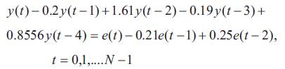
(1)
The most popular method of nonparametric spectral density is the Weighted Segment Overlap Averaging (WOSA). Because of the unequal weighting of observed samples, its variance estimate is non monotonic function of fraction of overlap. Simple theoretical analysis of the mean and the variance of the WOSA have been presented nicely. Selecting the optimal fraction of overlap, which minimizes the variance, is in general difficult since it depends on the window used. The main objective in this paper is to avoid the nonmonotonic behavior of the variance for the Welch Power Spectrum Estimator (PSE) by introducing circular overlap to the Welch method. With slight modification, the mean and the variance of Welch Circular Overlap Segment Averaging (WCOSA) have been presented. With the help of simulation, the performance evaluations of WOSA and WCOSA have been presented and finally, it is observed that the variance estimate based on WCOSA is a monotonically decreasing function of the fraction of overlap.
An important application area of Digital Signal Processing (DSP) is the power spectral estimation of periodic and random signals. There are mainly two classes of power spectrum estimators: the parametric and the nonparametric estimators. The parametric methods are model based and more accurate. In contrast to parametric methods, nonparametric methods do not make any assumptions on the data-generating process or model (e.g., autoregressive model, presence of a periodic component). There are five common nonparametric PSE available in the literature: the periodogram, the modified periodogram, Bartlett's method, Blackman–Tukey, and Welch's method. However, all these nonparametric PSE’s are modifications of the classical periodogram method introduced by Schuster (1978).
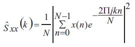
The periodogram is defined as
It is known that the periodogram is asymptotically unbiased but inconsistent because the variance does not tend to zero for large record lengths.
A way to enforce a decrease of the variance is averaging. Bartlett's method divides the signal of length N into K segments of length L = N/K each. The periodogram method is then applied to each of the K segments. The average of the resulting estimated power spectra is taken as the estimated power spectrum. Proakis & Manolakis (1996) views the variance is reduced by a factor K, but the spectral resolution is also decreased by a factor K. The Welch method eliminates the tradeoff between spectral resolution and variance in the Bartlett method by allowing the segments to overlap; see Figure 1. Essentially, the modified periodogram method is applied to each of the overlapping segments and averaged out.
The concept of windowing is applied to weight samples in an observation signal. The data window (taper) is used to attenuate the values of samples near the window boundaries in order to reduce some undesirable effects in the frequency domain. Due to discontinuities of data in the time domain causes the spectral leakage. The weighting of samples depends on the location of samples inside a data segment. For weak sense stationary signals, the unequal weighting is a not a problem, but for non stationary signals, like high amplitude transients, contain a lot of power in a relatively short time, if weighting is unequal, the location of the transient inside the data segment greatly affects the power estimate. Hence, the design of PSD estimates is of great importance concerning random signals and their analysis. Porat (1994) and Bronez (1992) were reported a drawback connected to the WOSA PSE: the variance is a nonmonotonically decreasing function of the fraction of overlap. The variance starts to grow when the fraction of overlap (exceeds 50%). This makes the method difficult to apply, as it is not clear which fraction of overlap to use since the optimum also depends on the type of the window used.
It is explained intuitively that this is a result of the competing effects of more segments (lowering the variance) and more overlap among segments (increasing the variance). In this paper, The authors show that this intuitive explanation does not hold. In particular, they illustrate that by using circular overlap in Figure 2, the variance of the PSE is monotonically decreasing as the fraction of overlap increases. The WOSA method suffers from the nonmonotonicity due to the unequal weighting of the measured samples, increasing the uncertainty of the PSE considerably. Furthermore, the variance of the PSE is reduced up to a factor K/(K-r), with the fraction of overlap r and the number of independent segments K, with respect to the variance of the Welch PSE. However, it is clear by using circular overlap that the concatenation of the end of the record with the beginning of the record, no extra systematic errors are introduced, implying that the circular overlap is asymptotically unbiased.
Brillinger (1975), and Stoica & Moses (1997) were shown that the Variance of the periodogram of an ergodic weakly stationary signal x(n) for n=0 : N-1 is asymptotically proportional to the square of the true power at frequency bin.
Welch (1967), Thomson (1982), and Harris (1978) suggested that the periodogram uses a rectangular time window, a weighting function to restrict the infinite time signal to a finite time horizon. A non rectangular time window in the modified periodogram.
Jokinen, Ollila, & Aumala (2000) reports the most efficient method of power spectral density (PSD) estimation is the WOSA or also called the Bartlett-Welch method.
Broersen (2006), Box & Jenkins (1970), and Porat (1994) presents the class of parametric PSE to fit a parametric model (AR, ARMA, MA, etc.) to the signal by minimizing a given cost function.
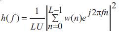
To compute an averaged periodogram estimate the signal has to be divided into K smaller units, called segments, which may overlap or be disjoint. Let x(n) is a sample from a wide sense stationary random process, having the length N For every segment a periodogram estimate is calculated. xi(n) consists of the samples of the ith segment, w(n) is a data window, where L denotes the number of data samples in a segment, 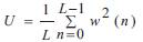 is a coefficient used to remove the window effect from the total signal power. For each segment of length L, the modified periodogram is defined from Welch (1967).
where,
then the WOSA power spectral density estimate is obtained by averaging K modified periodograms.
Overlapping changes the total weighting of data. At the boundaries of the data the weighting is always based on one coefficient. The other samples are weighted either by one or a sum of two or more coefficients of joined segments as shown in Figure1. When the overlapping is 50%, there are two or more coefficients summing up the weighting of each sample.
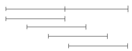
Figure 1. Regular overlap for K = 2 and fraction of overlap r = 2/3
The authors assume that the signal x(n) with n = 0,1,..., N - 1 is a weakly stationary Gaussian process. The signal x(n) is divided into K segments, such that every segment has length L = N/K further, they extract different overlapping subrecords by following the scheme of Figure 2. The overlapping subrecord of the signal x(n) satisfies
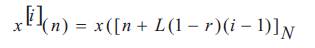
where n = 0,..., L - 1,0 r < 1and [n + L(1-r)(i-1)]N denotes n + L(1-r)(i-1)
modulo N imposing circular overlap. We need to impose that circular overlap implies an integer number of overlapping subrecords; further, the different subrecords need to overlap an integer number of time samples.
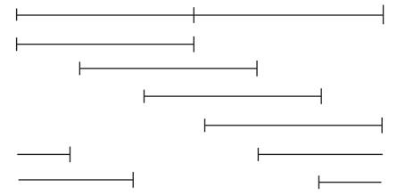
Figure 2. Circular overlap for K = 2 and fraction of overlap r = 2/3
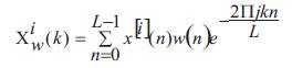
Barbe, Schoukens, & Pintelon (2008) were defines the windowed Discrete Fourier Transform (DFT) of the subrecord x[i](n) at frequency bin k as
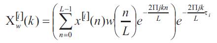
where τi (1-r) (i-1) L.
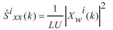
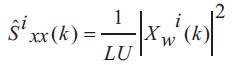
The proposed WCOSA method is applied for each subrecord as in Figure 2; the estimated power for subrecord xi(n) is defined as
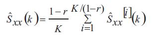
by averaging over the different overlapping subrecords in (5), an estimate of the power spectrum of the signal is defined as
From Welch (1967), the mean of WOSA is given by
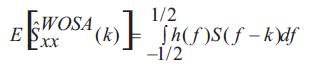
where
and the data window must satisfy
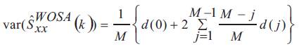
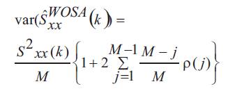
where M= (K-1)/ (1-r) +1 is the number overlapping subrecords for WOSA
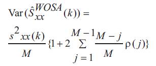
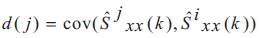
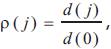
where
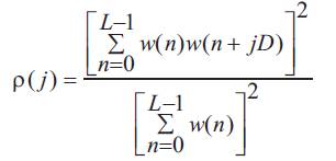
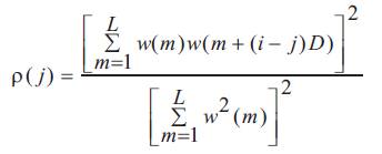
ρ(j) is a correlation coefficient and D is separation between two overlapped subrecords. The proof can be found in Appendix.
The mean of WCOSA is same as that of WOSA.
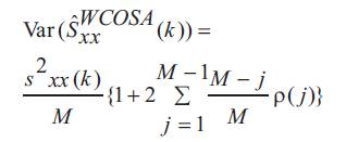
where M=K/ (1-r) is the number of subrecords in WCOSA.
Barbe, Pintelon, & Schoukens (2010) derived that the following inequality holds [9]:
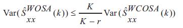
An important consequence of (13) is that the variance ![]() can be reduced as low as
can be reduced as low as ![]() Hence, circular overlap can reduce the variance of the WOSA up to factor 1-r/K.
Hence, circular overlap can reduce the variance of the WOSA up to factor 1-r/K.
The Signal x(n) with n = 0,1,..., N - 1 is a weakly stationary Gaussian process, such that x(n) = h(n) * e(n), where e(n) is zero-mean white Gaussian noise with unit variance and h(n) denotes the impulse response of the corresponding filter as shown in Figure 3. We assume that the sequence h(n) satisfies ![]()
The above implies that the filter characteristic H(ω) is continuously differentiable.
In this section, the method of circular overlap is illustrated as described in the previous section. In particular, the reduction in variance and the MSE are illustrated.
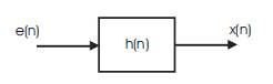
Figure 3. the Wold decomposition of weakly stationary signals
Keeping in mind the requirement of a maximal frequency resolution (e.g., system identification), we illustrate the method for K=2 (two data records only). We used a type 1 digital Chebyshev filter of order two, a pass band ripple of 20 dB, and a cutoff frequency at 0.15 x ƒs a zero-mean white Gaussian noise sequence with unit variance of N=2000 points was generated. The sequence was partitioned in two records of L=1000 points, and a Hanning window is applied. In Figure 4(a) the top plot shows the true power spectrum. The bottom plot the red curve shows ensemble average PSE of WCOSA, and the black curve shows ensemble average PSE of WOSA. The Figure 4(b) shows the corresponding root mean squared error (RMSE) of the WCOSA and WOSA, respectively, both estimated for 100 Monte Carlo simulations.
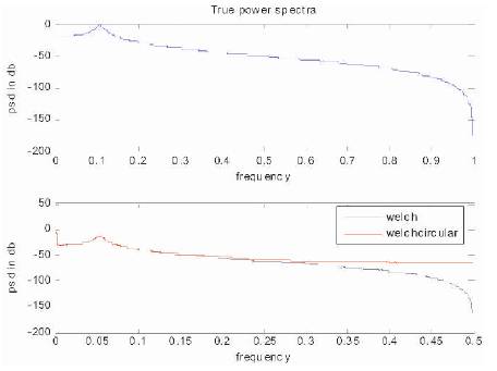
Figure 4(a). True power spectrum, PSE's of WOSA and WCOSA for chebyshev filter
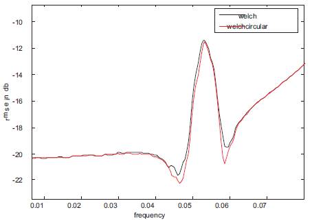
Figure 4(b). RMSEs of Welch and Welch circular
In Figure 5(b), we observe that we gain approximately 0.5 dB in RMSE in the pass band of the estimator, which is in agreement with a factor K/(K-r) of (13). However, for the higher frequencies, it is clear that the PSE of WCOSA has difficulties following the slope towards infinity, where the WOSA PSE does not suffer from this effect. Due to the fact that the variance of the PSE is proportional to the true power, the MSE for the higher frequencies is dominated by the bias contribution. They concluded that the variance of the WCOSA PSE is reduced, but at the expense of an increase in bias.
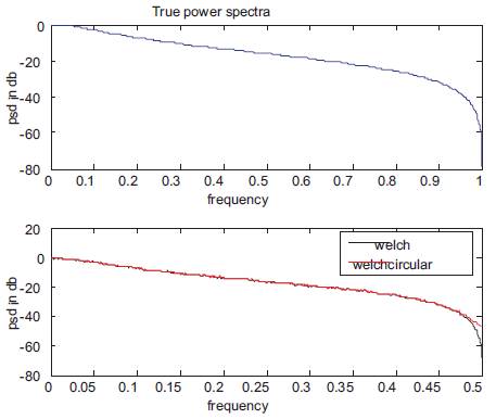
Figure 5(a). True power spectrum, PSEs of WOSA and WCOSA for butter worth filter
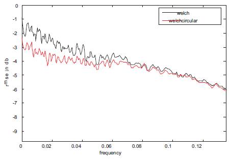
Figure 5(b). RMSE's of WOSA and WCOSA
In this example, we used a digital Butterworth filter of order 1, a cut off frequency at 0.1 x ƒs. A zero-mean white Gaussian noise sequence with unit variance of N=2000 points was generated via Matlab. The sequence was partitioned in K=4 records of L=500 points, and a Hanning window is applied. In Figure 5(a) the top plot shows the true power spectrum and the bottom plot red curve shows ensemble average of the WCOSA PSE, and the black curve shows ensemble average of the WOSA PSE. The Figure 5(b) shows the corresponding Root Mean Squared Error (RMSE) of the WCOSA PSE and the WOSA PSE respectively, both estimated for 100 Monte Carlo simulations. However the bias is significantly smaller than in Figure 4. This can be possibly addressed to the roll off of the filter characteristics as the roll off of a first order is smaller than for a second order filter.
The number of samples in each realization is assumed as N=1000. The sequence was partitioned in K=4 records of L=250 points, and a Hanning window is applied. After performing 100 Monte Carlo Simulations, In Figure 6(a) the top plot shows the true power spectrum. The bottom plot the red curve shows ensemble average of the WCOSA PSE, and the black curve shows ensemble average of the WOSA PSE. The Figure 6(b) shows the corresponding root mean squared error (RMSE) of WCOSA and WOSA, respectively.
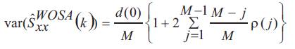
To illustrate monotonicity and nonmonotonicity of variance estimates i.e. equations (9) and (11) in WCOSA and WOSA as a function of the fraction of overlap r. In particular, the authors choose all fractions of overlap between 0.1 and 0.9. For the WOSA, the number of subrecords is an integer M= (K-1)/ (K-r) +1 and for the WCOSA, the number of subrecords is an integer M=K/ (K-r). Assume the number data samples is N=1000, the individual data segments K=2, the hanning window of length L= 500 is used. From Figure 7, it is observed that the variance estimate based on WCOSA is decreasing monotonically as function of fraction of overlap, unlike as that of WOSA.
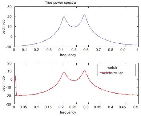
Figure 6(a). True power spectrum, PSEs of WOSA and WCOSA for ARMA narrowband process
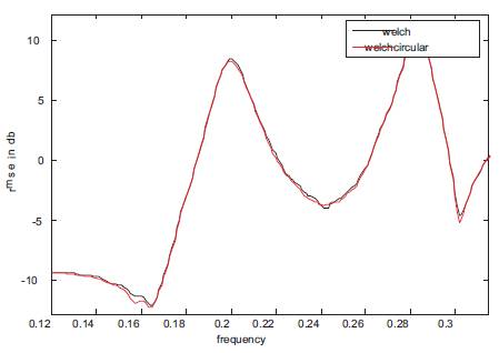
Figure 6(b). RMSE's of WOSA and WCOSA
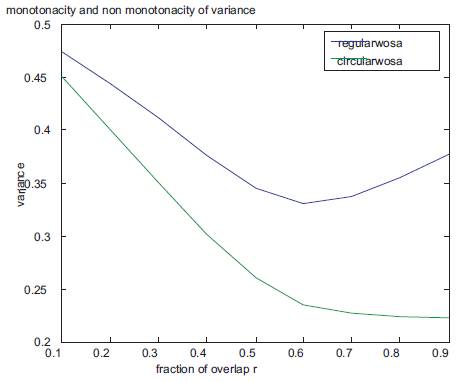
Figure 7. WOSA and WCOSA variance estimates vs. fraction of overlap r
In this paper, the reason for nonmonotonicity of the variance estimate in WOSA reported in the literature is exploited. The WCOSA method revealed that the nonmonotonicity of the variance of the WOSA is not due to the following tradeoff: increasing the fraction of overlap results in more subrecords to average but increases the correlation between two subrecords. The nonmonotonicity of the variance of the WOSA is due to the unequal weighting of the data, which implies that the covariance between two overlapping subrecords is weighted with a triangular window. The variance of the improved WCOSA is monotonically decreasing without introducing extra systematic errors. The WCOSA provides the user with a reduction of the variance with respect to the variance of the WOSA up to a factor K/(K-r) The numerical examples are simulated by using MATLAB 7.0.1 software.
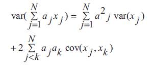
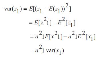
Assume N random variables x1, x2,........xN and its weights a1, a2,........aN, Papoulis (1965) presents the variance of sum of weighted random variables is given by
Proof: For j = 1, let Z1 = a1x1
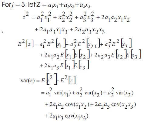
Similarly for j = N, let
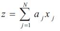
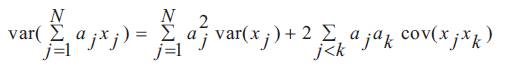
the end of the proof equation (15).
Proof of equation (9)
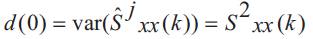
Let  and for WOSA, M is the number of overlapping subrecords, each having length L. With the help of equation (14), From Percival, & Walden (1993), the variance of WOSA power spectrum estimate is given by
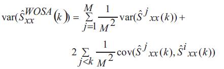
Then
where
Further if
then
Assuming x(n) is a sample from a Gaussian process and assuming Sxx(k) is flat over the pass band of the estimator,
and
Then
The proof of equation (11) i.e. the variance of WCOSA is obtained by replacing M in the equation (18) with  where K is number of segments and r is the fraction of overlap.