This paper presents how dispersion affects pulse propagation in the fiber. Dispersion is a fundamental property of the glass from which a fiber is formed. A fiber is dispersive because the index of refraction n and the propagation constant β are different at each optical frequency. The phase velocity of a wave with frequency ω is 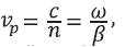 so the velocity also varies with frequency in a dispersive material. Since any data pulse is formed through the superposition of energy at different frequencies, digital pulses carried on an optical wave eventually break apart after propagating a sufficient distance. Mathematically, the effects of fiber dispersion are accounted for by expanding the mode propagation constant in a Taylor series about the center frequency ω_o [1],

(1)

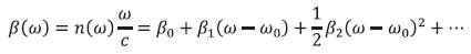
where,

(2)

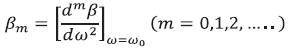
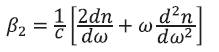
which describe how the propagation constant varies about the center frequency ω_o. The coefficients β_m are defined at ω_o. Here β₁ is related to the group velocity of ν_g the pulse in the fiber, and β₂ the dispersion coefficient that defines how rapidly a pulse spreads because of dispersion. To understand the concept of group velocity, let's consider the two waves with different frequencies. We simulate the behavior of two waves with different frequencies as seen in Figure 1(a). The superposition of the two waves

(3)

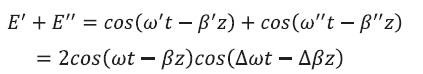
is depicted in Figure 1(b) at time The frequency ω is the average of ω’ and ω’’ and . Similarly frequency β is the average of β’ and β’’ and . If the frequencies of the two waves are similar, the difference (or beat) frequency Δω is small and the superposition consists of a higher frequency carrier wave cos(ωt-βz) that is modulated by a low frequency pulse envelope cos(Δωt-Δβz). The peak of the pulse envelops results where the two waves constructively interfere. In Figure 1(b) this is at z=0 as mentioned. The velocity of the carrier wave is the phase velocity . The velocity of the pulse envelope is the group velocity, . For a pulse composed of many frequency components,

(4)

where β₁ is the second term in the Taylor expansion of β. If  is different from the phase velocity of the carrier wave is different from the group velocity of the pulse envelop. Since  whenever the index n varies with frequency, as it does in dispersive material, v_g will be different from v_p. This is rather easy to describe mathematically. To physically see what is happening, we animate the two waves in Figure 1(a), each at a different phase velocity,  and  respectively. The group velocity of the pulse envelope is observed directly in the Figure 1(b). Initially at t = 0 in Figure 1(a), the crests of the waves coincide at z = 0. However in Figure 2(a), the two waves have moved 1.9µm and 2.0µm after 10 ƒsec, respectively. The phase velocity of the carrier wave is close to , between and so the carrier moves 1.95µm in 10 ƒsec.

In contrast, the pulse envelop in Figure 2(b) has shifted only slightly, so it moves a shorter distance in the same amount of time. Clearly, the pulse envelops moves at a slower velocity than the carrier wave. The reason lies in the fact that the envelope results from constructive interference between two waves. As the two waves move at different velocities, the phase position at which they constructively interfere moves at a velocity different from the individual phase velocities. Hence, the carrier wave appears to move through the pulse envelop as time progress. Real data pulses generally consist of more than two frequency components but the effect is precisely the same [2, 3].

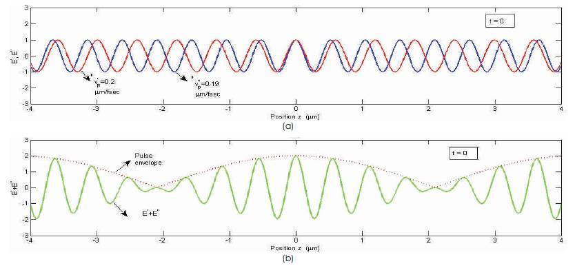
Figure 1(a). Two wave E’ and E’’ with different frequencies at t=0. b) Superposition E’+E’’ at t=0

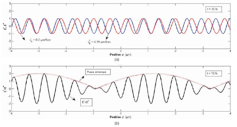
Figure 2(a). Two wave E’ and E’’ with different frequencies at t=10 fsec. b) Superposition E’+E’’ at t=10 fsec

As discussed in previous section, the pulse envelope moves at the group velocity  while the parameter β₂ is responsible for pulse broadening. The parameters β₁ and β₂ are related to the refractive index n and its derivatives through the relations

(5)

(6)

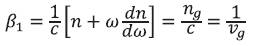
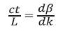
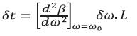
where n_g is the group velocity. The signal delay (propagation) time in an optical fiber around the center angular frequency ω_o is given by using equations (1) and (2),

(7)

(8)

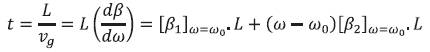
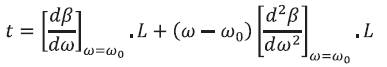
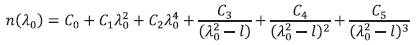
where L is the fiber length. When the signal delay time is different with respect to the different spectral components, which is caused by modulation or spectral broadening of the source itself, the signal waveform is distorted at the receiver end of the single mode fiber. In the multimode fiber, the group velocity itself may be different from mode to mode and this cause the pulse broadening. Multimode dispersion is the delay time dispersion caused by the difference of group velocity of the various modes. Polarization mode dispersion is a delay time difference between the orthogonally polarized HE^x_i1 and HE^y_i1 modes in the nominally single mode fibers or birefringent fibers. The slight birefringence in the single mode fiber is caused by the non concentricity of the core and the elliptical deformation of the core. Material dispersion is a delay time dispersion caused by the fact that the refractive index of the glass material changes in accordance with the change of the signal frequency. As we know that material dispersion is given by [4-5],

(9)

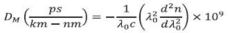
where λ_o is measured in µm and c = 3 x 10⁵ km/s. It is given

(10)

where
C₀ = 1.45,
C₁ = -0.003,
C₂ = -0.0000381,
C₃ = 0.0030,
C₄ = -0.0000779,
C₅ = 0.0000078,
l = 0.035.
From eq. (10) it can be shown as

(11)

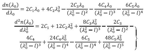
Plot of 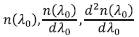 and D_m versus λ_o are shown in Figure 3 (a, b, c) respectively.

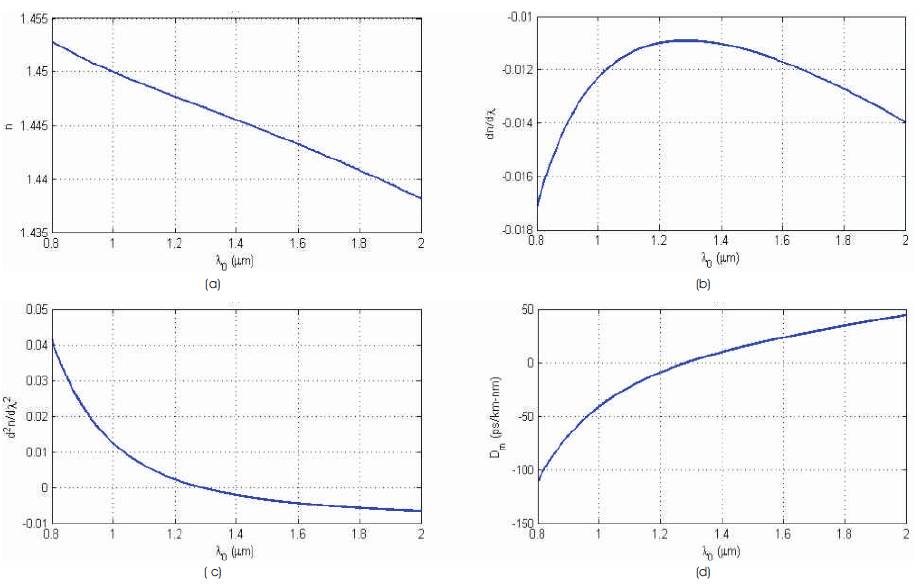
Figure 3. The index, group velocity, double derivative of index and group velocity dispersion in the near infrared region

Waveguide dispersion is a delay time dispersion caused by the confinement of light in the waveguide structure. The waveguide dispersion is an essential dispersion that inevitably exists in waveguides. Let us calculate the first term of eq. (8), which is related to the multimode dispersion. The delay time t in the fiber relative to the delay time in a vacuum, L/c is given by

(12)

When we consider a plane wave (propagation constant β_o) propagating in a homogeneous material of refractive index n the normalized delay time is expressed as [6],

(13)

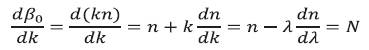
N is called the refractive index, since it is a function of both refractive index v_g through 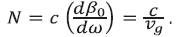. The propagation constant β is expressed in terms of the normalized propagation constant b as

(14)

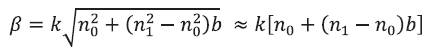
Substituting this equation into eq. (12) and by using eq. (13) it can be shown

(15)

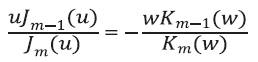
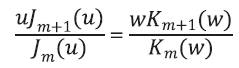
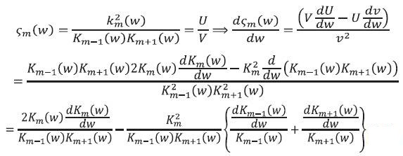
Here the researchers have used the fact that the difference between the core-cladding refractive index is almost the same as that between the group indices, we can approximate as . Next they have consider the calculation of . First the unified dispersion equation for the LP_ml mode is differentiated by v. Here it is expressed by reversing the denominator and numerator,

(16)

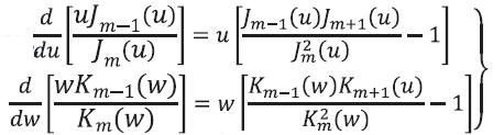
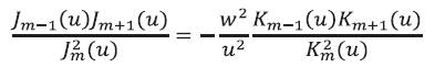
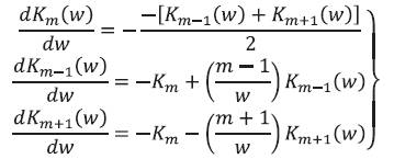
The differentiate of both terms in eq. (16) with respect to v gives [7],

(17)

(18)

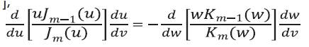
Now we can express eq. (16) in a different form

(19)

Combining equations (16) and (19), we obtain the relation

(20)

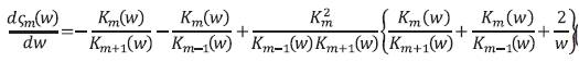
When we use the relation v² = u² + w² and equations (18- 20), into eq. (17), it is reduced to

(21)

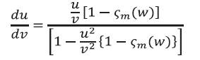
where

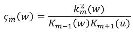
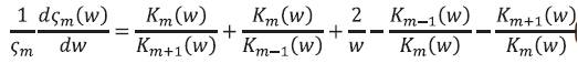
Considering the relation of  we obtain the expression  as

(22)

which can bet further simplified to get [8-10],

(23)

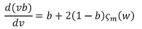
Figure 4 shows the dependence  for the few LP_ml modes on the normalized frequency v. The group delay or group velocity can be estimated by using equations (12) and (15) as

(24)

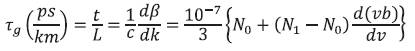
Figure 5 show the group velocity plot for LP₀₁ mode, similarly plot can be obtained for the other modes also. This study is useful to understand the group velocity dispersion concept.

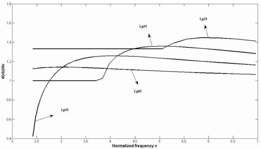
Figure 4. Normalized group delay for the step index fiber

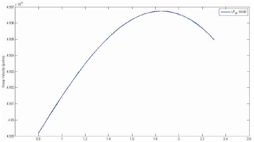
Figure 5. Group Delay  versus λ(µm) for LP₀₁ mode

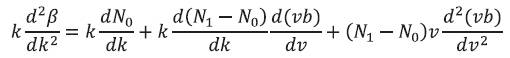
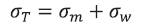
The sum of material dispersion and waveguide dispersion is called total dispersion or chromatic dispersion. Group velocity dispersion is given by eq. (8) as

(25)

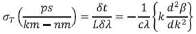
This equation can be rewritten using the relation ω = kc and as

(26)

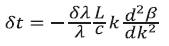
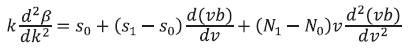
where δλ represent the relative spectral width of the signal source. Differentiation of eq. (15) by k gives

(27)

The derivative of the group index N given by eq. (13) with respect to k is then reduced to [11],

(28)

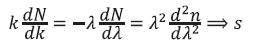
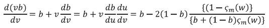
s is a normalized material dispersion and readily obtained by differentiating the refractive index n expressed by the Sellmeier polynomial. Figure 3(c) shows the normalized material dispersion plot. It is known that the material dispersion of silica based optical fiber becomes zero in the 1.3µm region. In eq. (27)  is obtained by differentiating eq. (23) by v and it may be calculated. Since from the eq. (23),

(29)

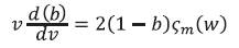
Hence

(30)

where . Now  can be found as follows,

(31)

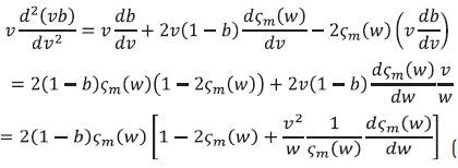
Now by using the following identity

(32)

Equation (31) leads

(33)

and also

(34)

Hence eq. (30) would transfer as

(35)

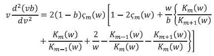
Figure 6, shows the normalized waveguide dispersion  of the LP₀₁ mode for a step index fiber.

Equation (27) can then be simplified to get [12-13],

(36)

The first term and second terms in right hand side of equation (36) represent the material dispersion and third term clearly represents the influence of the waveguide structure. Therefore, here the third term is defined as the waveguide dispersion. The total dispersion is usually expressed in terms of unit  spectral broadening per unit fiber length as

(37)

The total dispersion is then expressed as

(38)

where

(39)

(40)

For all practical purpose we can assume to first order  Hence

(41)

where . By using the eq. (10) it can be easily calculated and shown in Figure 3(d). In this paper for all the calculations we have considered to the first order

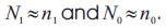
Figure 7, shows the effective indices versus wavelength for Lp₀₁ mode. Finally material dispersion, waveguide dispersion and total dispersion versus wavelength for LP₀₁ mode are shown in Figure 8. This Figure is corresponds to a = 3µm, n₁ = 1.476 and n₂ = 1.446 respectively. There is some percentage of error in the calculation due to approximation  in our calculation. Figure 9 shows the same plot but for different core radius. The zero total dispersion wavelengths come out to be

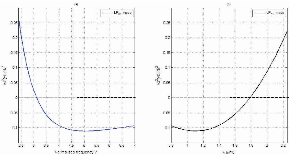
Figure 6. Normalized waveguide dispersion  versus a) normalized frequency and b) wavelength for the step index fiber

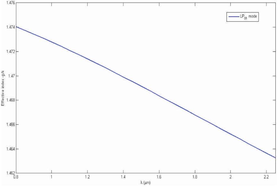
Figure 7. Effective indices  versus wavelength for LP₀₁ mode

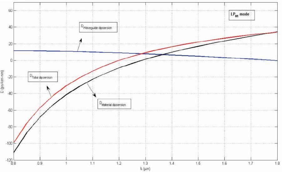
Figure 8. Material dispersion, Waveguide dispersion and Total dispersion versus wavelength for LP₀₁ mode

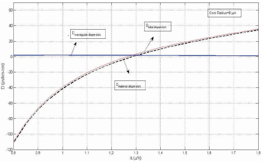
Figure 9. Material dispersion, Waveguide dispersion and Total dispersion (for a = 8 µm) versus wavelength for LP₀₁ mode

Waveguide dispersion study is useful in future to deploy of optical fiber link in WDM system. Researchers want to reduce the waveguide dispersion by tailoring the waveguide design parameters. However more complex waveguide structure shows more negative waveguide dispersion. In this paper, the authors have tried to compute analytical expression for  in terms of β. The detail calculations are presented into the paper. The study avoid of using numerical technique to calculate for waveguide dispersion. The simulation results found to be accurate enough for reasonable correct waveguide dispersion calculation. In addition presented technique in this paper can be easily extended to any other complex waveguide structure provided we must know the Eigen value equation.