(1)
Brain activity produces electroencephalogram signals, which consists of some of vital signs of neurological disorders and very much helpful in Brain Computer Interfacing(BCI). These signals can be acquired by placing the electrodes on the scalp at specified positions and exists in few hundreds micro volts range with a frequency band of DC-100 Hz. Acquisition of these signals is mainly suffers from different unwanted signals (noise) results in less signal information for identification. In this paper modeling of EEG signals has been done with wavelets and Iterative Soft Thresholding (IST)algorithm. Results reveal that the enhancement of these signals gives the exact features without losing the signal information.
EEG is one of the most effective diagnostic procedures for epilepsy and it is very helpful for research in Human Computer Interfacing (HCI). EEG records carr y information about abnormalities or responses to certain stimuli in the human brain. Some of the characteristics of these signals are the frequency and the morphology of their waves. These components are in the order of just a few up to 200 μV, and their frequency content differs among the different neurological rhythms, such as, alpha, beta, delta and theta rhythms [1]. However, artifacts and noise are the outstanding enemies of high quality EEG signals. Their presence is thus crucial for the accurate evaluation of EEG signal. They fall into two major categories: technical and physiological artifacts. The technical artifacts are often found in power line noise 50/60Hz results from poor electrode application on the scalp and tranducer's artifacts. The physiological artifacts are often due to ocular, heart and muscular activity; are the EMG, EOG and ECG artifacts respectively [2]. which are described below by its type.
Generally the electrical activity of the heart, as reflected by the ECG, can interfere with the EEG. Although the amplitude of the cardiac activity is usually low on the scalp in comparison to the EEG amplitude (1-2 and 20- 100 uV, respectively), it can hamper the EEG considerably at certain electrode positions and for certain body shapes [3]. The repetitive, regularly occurring waveform pattern which characterizes the normal heartbeats fortunately helps to reveal the presence of this artifact. However, the spike-shaped ECG waveforms can sometimes be mistaken for epileptic form activity when the ECG is barely visible in the EEG.
Secondly, noise generated with muscle activity is common artifact caused by electrical activity of contracting muscles measured on the body surface by the EMG [4]. This type of artifact is primarily encountered when the patient is awake and occurs during swallowing, grimacing, chewing, talking, sucking, and hiccupping [5]. It is generally occurring noise with Eye movement and blinks at the time of acquiring. Eye movement produces electrical activity, the EOG which is strong enough to be clearly visible in the EEG. The EOG reflects the potential difference between the cornea and the retina which changes during eye movement. Another common artifact is caused by eyelid movement ("blinks") which also influences the corneal-retinal potential difference. The blinking artifact usually produces a more abruptly changing waveform than eye movement, and, accordingly, the blinking artifact contains more high- frequency components [6].
This paper describes a novel method for signal enhancement of the active channels using wavelet based method with a iterative soft Thresholding algorithm. Fist signal is decomposed into 6 levels, all the detail coefficients which are having more noise information are processed with the (IST) and results are compared with the parameters SNRI SNRO and PRD which are noticeably high compared to the previous methods.
The rest of the paper is organized as follows. Section 1 briefly reviews the wavelet transform, section 2 presents the iterative soft thresholding and section 3 gives the details proposed procedure involving in enhancement of the signals using wavelet transform thresholding (IST). Finally, results and discussion given in section 4, conclusions are made in the last section.
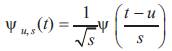
Wavelet analysis is becoming a common tool for analyzing localized variations of power within a time series. By decomposing a time series into time-series into time-frequency space, one is able to determine both the dominant modes of variability and how these modes vary in time. Wavelet Transform can be represented as a linear transformation i.e. Y= WX, where X, Y are input and output of the transformation and W is orthogonal mother wavelet transformation matrix. Mother wavelet is defined as
Wavelets are oscillating functions of time that must satisfy several conditions: A wavelet ψ has zero time average and unit energy corresponds to orthonormality property of wavelets. The amplitudes of a wavelet have large fluctuations within a designated time period and extremely small values outside of that time while being band-limited in terms of their frequency content. The CWT of a signal f (t) can be calculated using equation
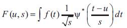
By varying the values for s and u results in an infinite number of combinations, can be used to decompose the signal f (t). Here u and s are the translation and dilation respectively.
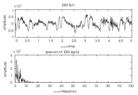
Figure 1. Original EEG signal in top trace and its spectrum in bottom trace
A much more computationally efficient approach is the use of the Discrete Wavelet Transform (DWT), which was developed by Mallat [7]. Knowing only the values of the DWT coefficients, the waveform can be perfectly reconstructed. All of the extra coefficients of the CWT create a redundancy in calculation because they are highly correlated with the ones of the DWT. In implementation, the DWT performs even better because waveforms are already digitally sampled and have finite duration so the number of coefficients is limited in DWT or CWT can be seen as a number on the time scale plane representing the correlation between the signal vector and the wavelet function at a given time-scale point. The DWT produces as many wavelet coefficients as there are samples in the original signal by using a filter scheme shown in Figure 1.
The original signal is convolved with a low and high pass filter whose impulse response is determined by the wavelet chosen. The output of each filter produces the same number of samples as the original signal, so both outputs are down sampled by 2 resulting in the approximation and detail coefficients each with half the number of points as the original signal.
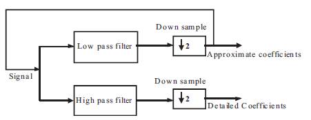
Figure 2. Block diagram to show the DWT decomposition
The coefficients represent a correlation between the signal of interest and wavelet chosen at different scales and during translation. Because all of the coefficients are preser ved, the original signal or any level of decomposition can be reconstructed using a filter scheme similar to decomposition shown in Figure 2. The process is reversed and now the coefficients are up sampled (interpolated), filtered, and summed.
EEG signal is decomposed into 4 levels using Daubenchies-4 (dB4) wavelet as mother wavelet Approximation and Detail coefficients are shown in the Figure 4.
From derived coefficients high frequency components will be distributed in approximate coefficients and low frequency components presents in Detail coefficients cD4, cD3, cD2, cD1.
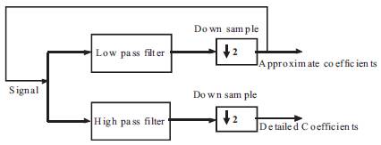
Figure 3. Block diagram to show the DWT reconstruction
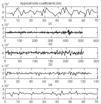
Figure 4. Approximate and Detail coefficients of EEG with 4 level decomposition
In this work we considered only detail coefficient cD4 for modeling EEG signals with wavelets. These cD4 coefficients are scaled with Iterative Soft Thresholding algorithm.
This method describes an approach for the restoration of degraded signals using sparsity. This approach, which has become quite popular, is useful for numerous problems in signal processing: denoising, de convolution, interpolation, super-resolution, de clipping, etc [6]. We assume that the observed signal y can be written as
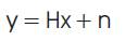
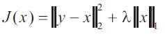
where x is the signal of interest which we want to estimate, n is additive noise, and H is a matrix representing the observation processes. For example, if we observe a blurred version of x then H will be a convolution matrix. The estimation of x from y can be viewed as a linear inverse problem. A standard approach to solve linear inverse problems is to define a suitable objective function J(x) and to find the signal x minimizing J(x).
Generally, the chosen objective function is the sum of two terms:
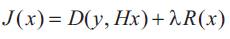
Where D(y, Hx) measures the discrepancy between y and x and R(x) is a regularization term (or penalty function). The parameter λ is called the regularization parameter and is used to adjust the trade-o between the two terms; λ should be a positive value. On one hand, we want to find a signal x so that Hx is very similar to y; that is, we want to find a signal x which is consistent with the observed data y. For D(y; Hx), we will use the mean square error, namely
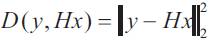
The notation  represents the sum of squares of the vector v
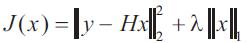
Objective function for soft thresholding can be considered as
This is a special simple case with H = I from the previous Expression
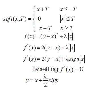
The objective function minimization form the previous Case
This J(x) can be minimized by combining MM approach, we wish to find a majorizer of J(x) which coincides with J(x) at xk and which is easily minimized. Adding non negative function to J(x)

By design, Gk(x) coincides with J(x) at xk . We need to minimize Gk(x) to get xk+1 . With above equation, we obtain

We can rewrite the equation using soft thresholding as Follows

where K is a constant with respect to x. Minimizing Gk(x) is equivalent to minimizing  so xk+1 is obtained by minimizing
Therefore minimizing is achieved by the following softthresholding equation:
Here in this paper we utilized the iterative soft thresholding algorithm for denoising the EEG signal. The model consisting of three main steps i.e, normalization, wavelet decomposition and applying the IST for the detail coefficients. In this paper EEG signals are taken from Physionet database.
Data can be normalized to increase the accuracy of the application as follow:
It is very important because of possible variations in signal acquisition from trial to trial, the normalization of data is necessary for valid results.
EEG data is decomposed into 4 levels using dB4 wavelet as shown in Figure 5 and all the detail coefficients are scaled by IST algorithm, finally by applying inverse wavelet transform results the enhanced EEG signal. Algorithmic flow results are shown in Figure 6 reveals that the presented method of modeling gives the good performance among all the previous techniques.
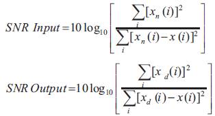
Where xn(i) is the noisy EOG signal,
xd(i) is the de noised EOG signal
x (i) is the Original EOG signal.
SNRI is defined as difference between SNR output and SNR inputs. Absolute Average Error (AAE) is average error.
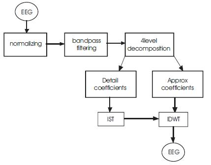
Figure 5. Algorithm flow
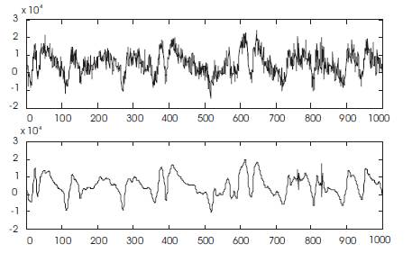
Figure 6. Original and modeled EEG signals
SNRi, SNRo, AAE are calculated with different mother wavelets and simulations are tabulated in Table 1.
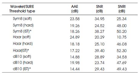
Table 1. Statistical measures for denoising using different wavelets
Iterative Soft Thresholding can be effectively utilised for denoising, super resolution and blind de convolution. When compared to soft thresholding, hard thresholding and adaptive techniques, IST provides good Signal to Noise Ratio (SNR), Absolute Average Error (AAE) and Relative entropy with the original signal. Hence it could be used efficiently for feature extraction in signal processing domain. The results shown in Table 1, clearly shows that IST is efficient than soft thresholding, hard thresholding and adaptive techniques.
The analysis is made on real-time data which was obtained from http://physionet.ph.biu.ac.il/physiobank/database