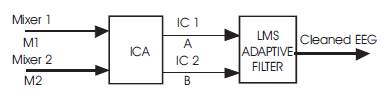
Figure 1. Model
Electroencephalogram (EEG) is used for the analysis of brain signals obtained from various electrodes placed across the scalp at specific positions. The collected signals from brain are often contaminated with Ocular Artifacts (OAs), EKG and EMG artifacts. In this paper a novel technique is used for the removal of ocular artifacts using FastICA algorithm which decomposes the EEG signals into independent components then an LMS (Least Mean Squares) based adaptive algorithm is applied to the independent components so as to get the original EEG signals. In the first step, independent basis functions attributed to OA are computed using FastICA algorithm. In the second step we arrive ocular artifact free EEG signal efficiently comparative to FastICA. This paper based on some parameters like Root Mean Square Deviation (RMSD) and Root Mean Square Variance (RMSV) we can say that the EEG signal obtained after second step is better than after the first.
The Electroencephalogram is a noninvasive facility to investigate the brain activity. Generally EEG signals falls in the range of dc to 100Hz classifying into alpha,theta,delta and beta waves[1]. The EEG is very susceptible to various activities like ocular artifacts due to eye movements and eye blinks. Magnitudes of OAs can be greater than of brain signal potentials, hence they can be clearly hinder the interpretation of EEG recordings. We require an artifact free EEG signal as it is needed.
Principal component analysis is also used to remove OAs in the recent years, but this analysis is not suitable for artifact removal especially when the amplitudes of artifacts is about equal to that of actual signals.
Blind Source Separation (BSS) methods have been widely used to extract the EEG signals contaminated with ocular artifacts blindly[2], [3], [4]. Independent Component Analysis (ICA) is a BSS method that blindly separates mixtures of independent source signals. ICA distinguishes with the other methods as it looks for the components which are statistically independent and non-Gaussian[5],[6],[7].Fast independent component analysis (FastICA) algorithm is an extended version of independent component analysis, with which the results can be obtained quickly, as computational efficiency is better[8],
Important applications of ICA include biomedical signal processing (usually brain wave activity in the form of EEG and MEG tracings), audio signal separation(mixed speech and music signals), telecommunications(a confusion of signals transmitted by multiple users of mobile phones), financial time series(portfolios of stocks), and data mining (text document analysis).
Linear filtering is required in a variety of applications. A filter will be optimal only if it is designed with some knowledge about the input data. If this information is not known, then adaptive filters are used. The adjustable parameters in the filter are assigned with values based on the estimated statistical nature of the signals. So, these filters are adaptive to the changing environment. In the proposed method LMS adaptive filtering is used as we don't have knowledge of quantity of ocular artifacts.
By applying the FastICA algorithm, we obtained the independent components (EEG and EOG) assuming statistically independent from available EEG signals. we then calculated the RMSD and RMSV values of the independent components[9], [10], [11] [9-11].The output of Fast ICA is applied to LMS adaptive filter to get the better RMSD and RMSV values compared to FastICA[8]. The comparison table shows the performance evaluation and is given in Table 1.
In this paper, for the decomposition of EEG data FastICA was applied. FastICA is one of the prominent approach with which we can remove the noise like ocular artifacts present in the EEG signals. The proposed model is shown as following:

Where, Matrix X is an observed signal, the row vector of X is Xi = ai1 S1 + ai2 S2 +.........+ ain Sn , for all i=1,…….n. S is an independent original signal. The elements of S are s1 ,s2 ,…..sn .and A is a mixing matrix with real coefficients. The elements of A are aij ,i,j=1,……n. ICA estimates the mixing matrix A with the observed signal X to get independent source S by inverse operation

The FasICA algorithm is described below:
1. Center the data to make its mean zero, then whiten the result to get X.
2. According to the formula
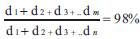
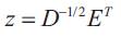
choose m Eigen vectors, then whiten the data to get Z using formula
3. Initial the separate matrix W, for every wi ,i = 1,......, m unit of norm. Orthogonalise matrix W as in step 5.
4. For all wi ,i = 1,......, m Let
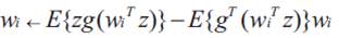
To renew wi generally we chose g(.) as hyperbolic tangent function.
5. Do a symmetric orthogonalisation of the matrix W = (w1 ......., wm )T by W ←(WWT )-½ W or by the iterative algorithm.
6. Iterate between step 4 and step 5, stop if convergence is attained.
Symmetric orthogonalisation is done by first doing the iterative step of the one-unit algorithm on every vector wi, in parallel, then orthogonalise all the wi by special , symmetric methods. After all the iterations W can separate the observed signal into independent source components and mixing matrix A. (AW-1 )
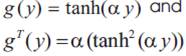
Where 1 ≤α≤2
Inputs: two mixer signals (M1 and M2) both containing EEG contaminated with EOG
Outputs: separated EEG and EOG assuming statistical independence.
Here the available EEG data EOG may or may not be Gaussian but are assumed to be statistically independent. Hence we cannot say that the obtained EEG data is a cleaned EOG. So to get the cleaned EEG data we go for adaptive filters which are used when the information about the inputs is not known.
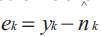
The LMS Adaptive Algorithm is described below.
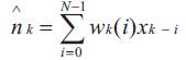
Initially, set each weight wk(i),i = 0,1,......, N-1, to an arbitrary fixed value, such as 0.
For each subsequent sampling instant k = 1,2,......, carry out steps (2) to (4) given below.
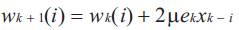
Inputs: independent components(EEG and EOG)
Outputs: cleaned EEG.
The data sets are collected from the website http://www.physionet.org. The data sets namely A and B,A corresponds to EEG contaminated with EOG and B corresponds to EOG,which are then linearly mixed, to get two mixers M1 and M2,which are taken as inputs to the ICA algorithm, as shown in Figure 1. The ICA algorithm works on these two mixers M1 and M2 and produces two independent components IC 1 and IC 2.
IC 1: Separated EEG signal (EEG+EOG) from the mixers
IC 2: Separated EOG signal from the mixers
Figure 1. Model
Then RMSD, RMSV are calculated for IC 1. Out of these two independent components IC 2 is used as reference signal and IC 1 is used as input signal to the LMS Adaptive filter. It gives the cleaned EEG signal from IC 1(EEG+EOG) taking IC 2 (EOG) as reference,as shown in Figure 2.
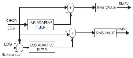
Figure 2. Flow Chart for Time Domain Measures
Root Mean Square Deviation (RMSD) and Root Mean Square Variation (RMSV) are used to assess the filtering efficacy and the degree of distortion of the signal after running the algorithms.
RMSD is the RMS value obtained from the pure EEG signal minus the restored EEG signal that has been processed by the adaptive filter. A smaller RMSD value indicates a better efficacy of the adaptive filter .
RMSV is the RMS value of the tiny variation from the original input EEG after it has been blindly processed by the algorithms. The RMSV indicates the degree of variation of the EEG signal processed by the adaptive filter.
RMSD is the Root Mean Square Deviation frequently used as a measure of the difference between the values predicted by a model or an estimator and the values actually observed from the thing being modeled or estimated. RMSD is a measure of precision. These individual differences are also called as residuals, and the RMSD serves to aggregate them into a single measure of predictive power.
RMSV is the Root Mean Square Variance
In the proposed method, RMSD and RMSV are calculated as follows:
for FastICA
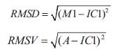
Where M1 is the available mixer signal, IC1 is the independent component 1 and EEG contaminated with EOG and the results of fast 1CA are shown in Figure 3.

Figure 3. Results of fast ICA: a)collected EEG b)collected EOG c) Mixer signal of (a),(b) d) Mixer signal of (a),(b) e) Obtained Independent component 1 (EEG) f) Obtained Independent component 2 (EOG)
For LMS Adaptive filter:
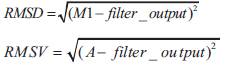
Where M1 is the available mixer signal, filter_output is nothing but cleaned EEG and A is EEG contaminate with EOG and the results of LMS Adaptive filter are shown in Figure 4. The results are tabulated in Table 1.
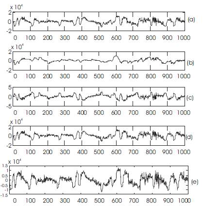
Figure 4. Results of LMS Adaptive Algorithm: a) Mixer of Mixer (a), (b) of Figure 3. b) Mixer of Mixer (a),(b) of Figure 3. c) Independent Component 1 as reference input to the filter d) mixer signal as input to the filter e) original EEG signal as input to the filter
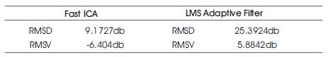
Table 1. Performance Measures
The majority of the proposed BSS-based AR techniques, concerns the identification of the artifactual components. All of them remove the artifactual components by zero-padding the proper elements in the mixing matrix and these techniques distorts the underlying neural activity.
Castellanos and Makarov[11]proposed a method which relies on ICA, and makes use of the wavelet theory for recovering the cerebral activity lying under the artifactual components. However, this method passes all the components through a thresholding procedure which cuts out only the high magnitude voltages (like eye blinks). This methodology suffers, especially in cases where high magnitude voltages are not derived from artifactual sources, but they are originated from true brain responses (like epileptic EEG signals). This approach overcomes this problem by employing adaptive filtering procedure (LMS) on EOG signals. Thus,only artifacts related with EOG activity are removed.
In this paper, FastICA is applied for removing the ocular artifacts in EEG, if the reference EOG signals are available. But it cannot remove all the ocular artifacts as it assumes the available EEG data as statistically independent. So, for the further removal of artifacts the obtained EEG signal is applied to the LMS Adaptive filter[12].
RMSV and RMSD parameters are calculated for the output (EEG+EOG) of FastICA and the output (cleaned EEG) of LMS Adaptive filter. The results, shown in Table 1 concludes that ocular artifacts can be better removed using this hybrid algorithm namelyFastICA-Adaptive(LMS)filtering algorithm.
The disadvantage with the proposed method is that it needs EOG as reference signal.
The proposed method suggests that the removal of ocular artifacts usingFastICA-Adaptive (LMS) algorithm is better than other ocular artifact removal methods or techniques.