This paper investigates the application of Unscented Kalman Filter (UKF) for Induction Motor (IM) sensorless drives. UKF's use nonlinear Unscented Transforms (UT) in the prediction step in order to preserve the stochastic characteristics of a nonlinear system. The advantage of using Uts is their ability to capture the nonlinear behavior of the system, unlike extended Kalman filters that use linearized models. Four original variants of the UKF for IM state estimation, based on different UTs are described, analyzed, and compared. The four transforms are basic, general, simplex, and spherical UTs. This paper discusses the theoretical aspects and implementation details of the four UKFs. It is concluded that the UKF is a viable and powerful tool for IM state estimation and that basic and general UTs give more accurate results than simplex and spherical UTs.

Accurate estimation of state variables of systems is very important for practical systems. Kalman Filter (KF) is most widely used for state estimation. The most common application of the KF to nonlinear systems is in the form of Extended KF(EKF). Linearization in EKF introduces errors in the corresponding state estimations. The linearization is performed usually by Taylor expansion and the error is due to neglecting higher order terms.

Although the EKF maintains the elegant and computationally efficient update form of KF, it suffers from number of serious limitations [1]. EKF is difficult to tune, the jacobian can be hard to derive, and it can only handle limited amount of nonlineariy. A nonlinear Kalman Filter which shows promise as an improvement over the EKF is the Unscented Kalman Filter (UKF) [2]. In the UKF, the probability density is approximated by a deterministic sampling of points which represent the underlying distribution as a Gaussian. The nonlinear transformations of these points are intended to be an estimation of the posterior distribution, the moments of which can then be derived from the transformed samples. The transformation is known as the Unscented Transformation (UT).The UKF tends to be more robust and more accurate than the EKF in its error estimation .

The paper is organized as follows. In section 1, the UT concept is discussed. In section 2, the UKF and the discrete UKFs are discussed. The IM model and observer are described in section 3. Comparisons of UKFs are described in section 4. Section 5 provides the simulation results. Conclusions and scope for future work are given in the last section.

It is difficult to characterize the output of a nonlinear system subject to a stochastic input. The simplest and most common approach to this problem is to linearize the system and obtain the stochastic output of the linearized model. Although this provides a good approximation in some cases, it can lead to inaccurate results. The UT is a nonlinear transform that provides a good characterization of the output of a nonlinear system subject to a stochastic input.

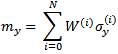
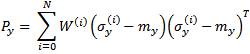
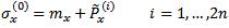
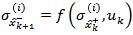
The different UTs are used to estimate the states of an IM. Suppose that we know the mean mx and covariance Px of a n × 1 stochastic vector x and moreover, suppose that we are interested in the mean and covariance of the output of a known nonlinear function y= h (x), A set of sigma points σ_x⁽ⁱ⁾, i = 0, 1, 2,……N, with the same mean and covariance as the vector can be selected. Then, the sigma points are transformed through the known nonlinear function h (x) to obtain a set of projected sigma points σ_x⁽ⁱ⁾ , i = 0, 1, 2,……N. The weighted sample mean and sample covariance of the projected sigma points give a good approximation of the true mean and covariance of the output y. If the weight associated with the ith sigma point is denoted by W(i) then the approximate mean and covariance of the output are calculated as:

(1)

(2)

In the basic UT, we choose the 2n sigma points

(3)

(4)

(5)

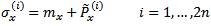
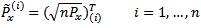
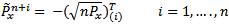
Where √nP_x is the matrix square root of nPx i.e.

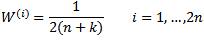
(√nP_x)^T √nP_x = nP_x and (√nP_x)_(i) is the ith row of √nP_x The square root of a matrix is calculated using the Cholesky factorization, which adds to the computational cost of the algorithm. However, the computational cost of Cholesky factorization is drastically reduced in the case of sparse matrices. The basic UT uses equal weights W⁽ⁱ⁾ = 1/2n i=1,…..,2n to calculate the mean of 4.1 and the covariance of 4.2. This reduces them to the conventional sample mean and covariance respectively.

The general UT uses a set of 2n+1 sigma points which lie on the √n^th covariance contour [6]. The authors refer to this choice as the general UT since it includes the basic UT as a special case. The general UT uses the 2n+1 sigma points

(6)

(7)

(8)

(9)

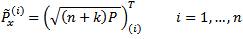
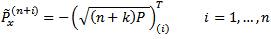
Unlike the basic UT, the sigma points are assigned unequal weights in the calculation of the mean and covariance as follows:

(10)

(11)

The design parameter k determines the degree of emphasis on point σ_x⁽⁰⁾, and reduces the higher-order approximation errors. For k = 0, the general UT reduces to basic UT.

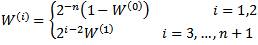
The number of the sigma points for the basic UT and general UT are 2n and 2n+1 respectively. To reduce the computational load, we must use fewer sigma points. At least n+1 sigma points are needed to capture the mean and covariance of a n×1 vector, and this is the number used in the simplex UT. The simplex sigma points are found using the following algorithm.

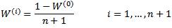
Choose a weight W ⁽⁰⁾ є [0, 1],

Choose the remaining weights as follows:

(12)

Initialize the 5 vectors as follows:

(13)

(14)

(15)

Expand each vector α(i), i =0,…., N recursively for j = 2,…..,n

(16)

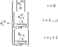
Use the -element vectors α ⁽ⁱ⁾, i =0,….,n+1 to determine the sigma points with

(17)

The third step of the algorithm sets the initial values of the first entry for α (i), i =0, 1, 2. In the fourth step, equation (4.16) iteratively determines the elements of each vector α (i). The α vectors are used in the final step to determine the sigma points.

Simplex UT uses n+2 sigma points, but the choice of W ⁽⁰⁾ = 0 reduces the number of sigma points to n+1. In general W⁽⁰⁾ is chosen by the user and it affects the fourth and higher order moments of the approximation.

The weights for simplex UT in (12) increase geometrically. For systems of high dimension, this can cause numerical problems, such as overflow or quantization errors. Therefore, while simplex UT saves computational time, it is not recommended for high dimensional nonlinear systems.

The spherical UT uses n+2 spherical sigma points. It therefore has the same computational cost as the simplex UT, but provides improved numerical stability. The algorithm for finding the spherical sigma points is similar to that for the simplex sigma points but with (12) replaced by

(18)

and (16) replaced by

(19)

Equation (18) shows that, unlike the simplex UT, the spherical UT uses equal weights. This is why the spherical UT is expected to have fewer numerical problems. Since the vectors in (16) and (19) are usually calculated offline, we expect the same computational load in processing the nonlinear transformations for simplex and spherical UTs.

The Unscented Kalman Filter belongs to a bigger class of filters called Sigma-Point Kalman Filters or Linear Regression Kalman Filters, which are using the statistical linearization technique [3,4].

The discrete KF uses the first two statistical moments and updates them with time. This is the key idea when combining the UT and KF to obtain UKF. The UKF is basically the discrete KF in which an UT is used to obtain the mean and covariance updates. The UKF as presented here is a simplified UKF which is suitable for estimation of IM states. In general, the observation model can also be nonlinear and all parameters and functions can be time-varying [7]. Moreover the UKF can be extended to the case of non-additive noise [8].

Given the discrete-time nonlinear system and a linear measurement model [5]

(20)

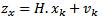
Where x_k is an n×1 state vector, Z_k is an m×1 measurement vector, H is the measurement matrix (m×m) and f (x_k, u_k) is a known nonlinear state transition vector. It is assumed that the process noise w_k is white and zero mean with covariance matrix Q and measurement noise v_k is also white and zero mean with covariance matrix R. Estimates of the initial state and the initial error covariance matrix P⁺₀ are available. The iterations in the classic KF consist of a prediction step followed by a correction step. For the correction step we use the discrete KF equations.

(21)

(22)

(23)

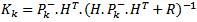
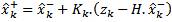
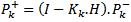
Where K_k is the Kalman gain.

The prediction step in the KF is the projection of the mean and covariance P⁺_k in time using the state equation. For the nonlinear system of (9), the state equation is a nonlinear transformation of a stochastic input x_k. Hence, the UT can be used to obtain the mean and covariance P^-_k+1 of its output.

The mean and the covariance P⁺_k of the stochastic input x_k are used to obtain a set of sigma points (I= 0, 1, 2,…., N) and the corresponding weights (W(i), i=0,1, ….., N). Then the sigma points are projected in time using the non linear transformation(9).

(24)

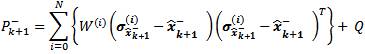
Given the projected sigma points we calculate the predicted mean using (1) and the predicted error covariance P^-_k+1 using the following modified version of (2)

(25)

Although the UKF is computationally costly, its computational load is acceptable for modern microprocessors. The most costly operations are the Cholesky factorization and outer products in obtaining the covariance of the projected sigma points. While the latter is an inevitable costly operation, Cholesky factorization can be simplified when the error covariance matrix is sparse. Since the load torque T_L appears only in the swing equation, its cross-correlation with both currents and both fluxes is negligible and it can be considered independent of both the currents and the fluxes. In addition, the orthogonality of the axes implies that φ_sα and φ_sβ are independent, as are i_sα and i_sβ. Consequently, the covariance matrix is sparse. For application to the IM, symbolic manipulation can be used to simplify the expressions off-line and thereby significantly reduce the computational load.

The IM state space model in the stator reference frame is

(26)

(27)

(28)

(29)

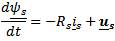
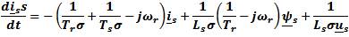
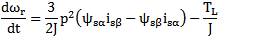
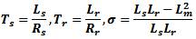
Where φ_s is stator flux space vector, i_s is stator current vector, p is the pole pairs, J is the inertia, R_s and R_r are the stator and rotor resistances, L_s and L_r are the stator and rotor inductances, and L_m is magnetizing inductance.

 

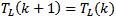
ω_r is the rotor speed, and u_s = u_sα+ j u_sβ is the stator voltage vector, which is the system input. The load torque is T_L, it is usually unknown, and in this model is assumed constant. The choice of stationary reference frame results in a simpler mathematical model and a simpler UKF design. However the UT is applicable to any state-space representation of the IM, in any reference frame, and is not limited to the one chosen here.

To use the discrete KF, we discretize the IM model by solving the system's state equation to determine the states at the sampling instants. To avoid cross-coupling problems, the authos use the forward Euler method which provides an acceptable approximation of the system dynamics for a short sampling period t_s. The resulting system is:

(30)

(31)

(32)

(33)

The state vector is chosen as

(34)

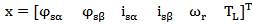
The stator current is the measured output and the measurement is

(35)

Thus, the measurement model is linear.

Based on Section I, the basic UKF is a special case of the general UKF, in which the original mean is not considered as a sigma point. Taking this sigma point into account will result in general UKF (with k = 1). Since all simulation results for basic and general UKF are almost identical, we only show the Simulation results for the general UKF.

To illustrate the UKFs performance in high speed operation with fast dynamics we show a startup followed by a reversal. The motor runs at zero speed, accelerates to 314 rad/s, and then reverses to -314 rad/s (electrical speed), all in a time span of less than one second. The simulation results for general UKF are shown in Figure 1 where we used thirteen sigma points and k = 1.

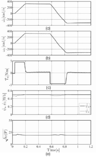
Figure 1. Simulation results for high speed operation of IM with general UKF (a) Estimated Speed, (b) Measured Speed, (c) Estimated Torque, (d) Estimated Stator and Rotor Flux Magnitudes, (e) Root Mean Square of Error

The simplex and spherical UKFs use the least number of sigma points but the latter is more numerically stable. The simplex UKF may lead to problems caused by overflow or underflow, and in the worst case it may even result in divergence. The simulation results for the simplex UKF with eight sigma points are shown in Figure 2.

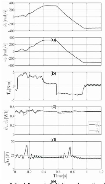
Figure 2. Simulation results for high speed operation of IM with simplex UKF (a) Estimated Speed, (b) Measured Speed, (c) Estimated Torque, (d) Estimated Stator and Rotor Flux Magnitudes, (e) Root Mean Square of Error

The simplex UKF gives poor speed estimation compared to the general UKFs. If the computational load is very critical, the simplex UKF may be selected over the general UKF, at the cost of a modest estimation performance. The spherical UKF is another computationally efficient filter but has better numerical accuracy because its weights are of the same order of magnitude. The simulation results with spherical UKF are shown in Figure 3 where we used eight sigma points. In high speed operation, the spherical UKF has similar performance as the general UKF. However some tracking errors are observed during speed startup.

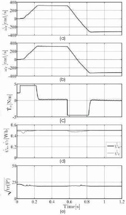
Figure 3. Simulation results for high speed operation of IM with spherical UKF (a) Estimated speed, (b) Measured speed, (c) Estimated torque, (d) Estimated stator and Rotor flux magnitudes, (e) Root mean Square of Error

The simulation results for high and low speed operation show that the general and basic UKFs have better performance than the simplex and spherical UKFs. Therefore, the author only evaluate the very low speed performance of general UKF. The authors test two speed profiles: square and triangular speed reference.

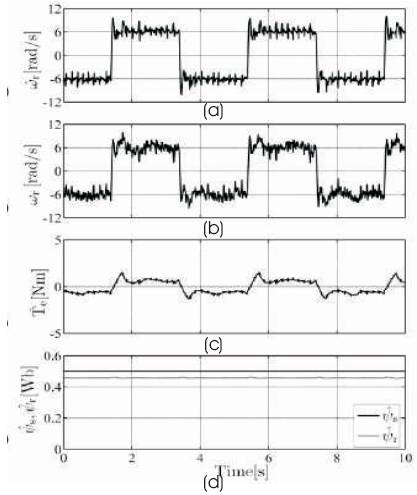
Figure 4. Simulation results for low speed operation of IM with square speed reference of 6.283rad/s and general UKF (a) Estimated speed, (b) Measured speed, (c) Estimated torque, (d) Estimated stator and rotor flux magnitudes

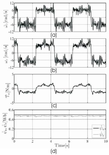
Figure 5. Simulation results for low speed operation of IM with square speed command of 6.283rad/s and spherical UKF (a) Estimated speed, (b) Measured speed, (c) Estimated torque, (d) Estimated stator and rotor flux magnitudes

IM observers based on fundamental excitation models, like the one we use here, are difficult to operate at speeds close to zero stator frequency where the drive becomes unstable [9]. It is therefore harder to track a triangular command that slowly crosses the instability region. Figure 6 shows the estimation results of the general UKF in slow reversal operation. Clearly, the observer is able to handle this situation well.

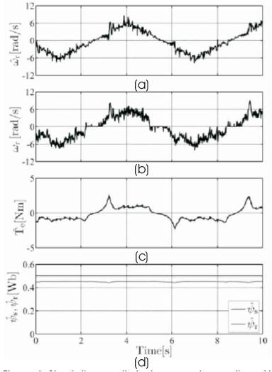
Figure 6. Simulation results for low speed operation of IM with triangular speed command of 6.283rad/s and general UKF (a) Estimated speed, (b) Measured speed, (c) Estimated torque, (d) Estimated stator and rotor flux magnitudes

For Figure 7 the author use the square wave speed command with 0.6 Hz amplitude. Below this speed, the dynamic response deteriorates abruptly and the drive cannot follow the reference speed.

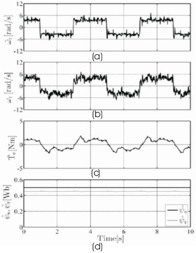
Figure 7. Simulation results for low speed operation of IM with square speed command of 3.77rad/s and general UKF (a) Estimated speed, (b) Measured speed, ( c) Estimated torque, (d) Estimated stator and rotor flux magnitudes

This paper proposes a family of unscented Kalman filters for IM drives state estimation. The original contribution is the investigation, application, and comparison of four UKFs that use four unscented transforms: basic, general, simplex and spherical. The comparison includes results for low speed operation of the drive. The four unscented observers are proposed and compared in this paper.

The basic and general UKFs display identical performance. They provide fast and accurate enough estimation over a wide speed range. Although the overall performance of the spherical UKF is inferior to that of the basic and general UKFs; its high speed operation is similar to that of the basic and general UKFs. Low speed operation suffers from larger errors than the basic and general UKFs.

The simplex UKF displays poor performance at low speeds and during fast transients. This disqualifies it from application in IM drives. In addition, the computation time for simplex and spherical UKFs is larger than for general UKF, which makes them less attractive for practical use.

The IM name plate data and parameters are: P_N=0.75hp, U_SN=240V, f_SN=60HZ, n_N=1725rpm, p=2, T_eN=3.1Nm, R_s=2.3Ω, R_r=2.5Ω, L_s=L_r=0.25H and L_m =0.24H.

The noise covariance matrices used are Q=diag{1.3x 10^-6, 1.3x 10^-6,1.4x10^-5, 1.4x10^-5,5.17x10^-7} and R=diag{120,120} and the initial setting is selected as a zero-mean vector with an identity error covariance matrix.