Radar is the most common sensor used in many applications such as imaging, missile guidance, remote sensing and global positioning. Synthetic Aperture Radar (SAR) is a valuable resource in remote sensing with varied scope in environmental, technological and military applications. SAR was first proposed by Carl Wiley (1954) wherein he describes the use of Doppler Frequency analysis to improve radar image resolution in M. Y. Chua and V. C. Koo (2009). In conventional radar systems, image resolution is dependent on the size of the illumination footprint on ground. Current strip-map SAR systems use pulsed FM waveforms to produce the radar signal. This technique results in complexity while designing the system. FM-CW is a technique used in many radar systems to achieve high pulse compression and large processing gains. This is based on transmission of Linear Frequency Modulation (LFM) signals and consideration of Doppler frequency shifts in received signals.

Unmanned Aerial Vehicle (UAV) is an aircraft that is capable of operating without the presence of pilot or crew in the aircraft. It is employed extensively in the area of reconnaissance and surveillance as well as for military purposes in Taylor A. J. P. (1977). In recent years, the usage of UAV in research area is growing rapidly and it has become an alternative platform for SAR. As compared to conventional airborne or space-borne SAR system, UAV based SAR has lower operation cost, lower risk, and is suitable for in-situ measurement where frequent revisit is required as cited in Duersch M. I. (Dec-2004).

Micro-SAR (μSAR) is ideally suited to be flown in a UAV due to suitability of design as compact, light-weight and lowcost radar. It also improves over previous SAR designs with regard to power consumption and therefore, can be developed with the specific goal of consuming less than 20 Watts (cited in Duersch M. I., Dec-2004).

Range resolution may be obtained using pulses of very short transmit duration. The resolution resulting from a simple square pulse shape with duration T is

(1)

Iin meters per pixel, where Δr is range resolution and c is the speed of light. Consequently, shorter the pulse length, finer the resolution in range. Taking this to the logical limit suggests a delta function as the pulse shape. Unfortunately, this ideal pulse is impossible as the delta function has infinite magnitude. In practice, hardware designed to transmit pulses of very short length is expensive and such systems suffer from low signal to- noise ratio (SNR). To alleviate this, it is possible to obtain high resolution using longer pulses that are frequency modulated. Linear frequency modulation (LFM) is by far the most common signal type used in practical SAR applications (W. G. Carrara, 1995).

An LFM chirp is a sinusoidal signal with linearly varying frequency. A complex LFM chirp can be written as exp(jπβt²) where β is the chirp rate. The time derivative of this phase term gives the frequency 2πβt, a linear function in time. Multiplying by a time-shifted copy of its conjugate (matched filter) results in a signal with linear phase whose frequency is proportional to the time shift. There are several different methods for deriving the range resolution of an LFM chirp (Adam E. Robertson, 1998; M. Soumekh, 1999; G. Franceschetti & R. Lanari, 1999); however, one simple approach is to recognize that radar bandwidth is approximately equal to 1/T, and therefore, Eq. (1) can be expressed as

(2)

where BW is the bandwidth of the transmitted signal. Increasing the transmit bandwidth thus improves the resolution. This result is consistent with various derivations, and is a common rule-of-thumb in SAR signal processing.

As discussed above, the type signal used in transmission is crucial to obtaining the benefits seen in SAR imaging. Improved resolution in the range direction is achieved through use of an LFM transmit signal. There are two types of LFM signals used in SAR, pulsed and continuous wave. Typical transmit signals for pulsed and continuous-wave radars are shown in Figure 1(a) and (b) respectively.

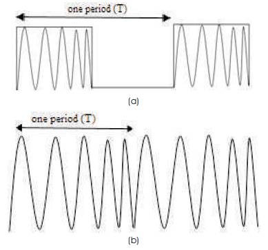
Figure 1. (a) Pulsed radar, (b) Continuous-wave radar

Pulsed signal transmission is employed by traditional SAR systems and is by far the most commonly used. It involves transmitting a quick burst of electromagnetic radiation and recording the received reflections off landscape targets, then waiting a short period of time and repeating the process. The term, Pulse Repetition Interval (PRI) refers to the elapsed time between pulse transmissions. PRF refers to the number of pulses transmitted per second, and is equal to the reciprocal of PRI.

Linear frequency modulation continuous-wave (LFM-CW) radar, on the other hand, transmits continuously and receives simultaneously. Although the signal is continually being transmitted in LFM-CW radar, it is possible to draw an analogy between pulsed and LFM-CW methods. As seen in Figure 1(b), frequency of the transmit signal increases, then decreases, then increases again and so on. Time taken for the frequency oscillation to ramp up and back down is considered as the PRI, and hence the number of up/down ramps per second is the PRF.

Figure 2 shows the LFM-CW transmit/receive model of frequency versus time. Received returns off targets are time delayed, (t0...tn) transmit signals. Targets further in range correspond to a greater frequency difference. In the figure, T represents the duration of one up-ramp, or half the PRI.

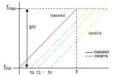
Figure 2. Showing LFM-CW signal return off multiple targets

A key difference between the two types of SAR is that pulsed radar generally mixes the received signal down to some intermediate frequency, then samples and stores the data, while LFM-CW radar mixes the received signal with the transmitting signal (this process is known as dechirping - essentially a delayed copy of itself), and then samples. This has the advantage of requiring a lower sampling frequency, but the disadvantage is the requirement of a higher dynamic sampling range.

LFM-CW radar also has the advantage of consuming less power than pulsed radar. This is because LFM-CW transmits pulses of much longer duration. Longer pulse length yields more energy contained in a single pulse; hence, LFM-CW SAR transmits with less power to maintain the same SNR as conventional, pulsed SAR. Since μSAR must operate with low power and cost requirements to be suitable for a UAV, an LFM-CW transmit signal is a better option. An LFM-CW also simplifies the sampling hardware and lowers the overall cost and size of the system.

In this paper, generation of chirp signal is done using DDS (Digital Direct Synthesizer). DDS can be designed in different ways like Look Up Table (LUT) based DDS, Coordinate Rotation Digital Computer (CORDIC) algorithm based DDS and Infinite Impulse Response (IIR) based DDS.

The basic block diagram of a direct digital frequency synthesizer (http://www.analog.com, 2011) is shown in Figure 3.

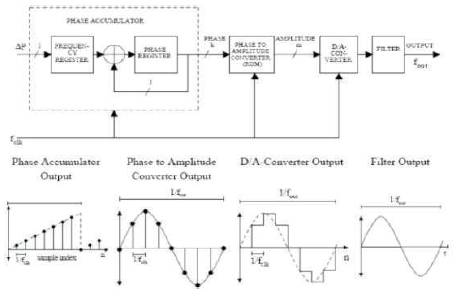
Figure 3. A simple block diagram of digital direct synthesizer and the signal flow in the DDS

As shown in Figure 3,the main components of a DDS are a phase accumulator, phase to-amplitude converter (a sine look-up table), a digital-to-analog converter and filter. A DDS produces a sine wave at a given frequency. The frequency depends on three variables, the reference clock frequency (fclk), the binary number programmed into the phase register (Frequency Control Word, M) and length of N-bit accumulator. The binary number in the phase register provides the main input to the phase accumulator. If a sine look-up table is used, the phase accumulator computes a phase (angle) address for the look-up table, which outputs the digital value of amplitude corresponding to the sine of that phase angle to the Digital to Analog Converter (DAC). The DAC, in turn, converts that number to a corresponding value of analog voltage or current. To generate a fixed frequency sine wave, a constant value (the phase increment that is determined by the binary number M) is added to the phase accumulator with each clock cycle. If the phase increment is large, the phase accumulator will step quickly through the sine lookup table and thus generate a high frequency sine wave. If the phase increment is small, the phase accumulator will take many more steps, accordingly generating a slower waveform (http://www.analog.com, 2011).

(3)

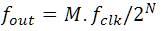
The above equation is known as the DDS frequency generating equation. The frequency resolution of the system is equal to f_clk/2^N. Implementation of DDS design in FPGA using LUT is shown in Figure 4(a) and the results of the same are shown in Figure 4(b). The model is simulated and implemented using System Generator blocks in Simulink. The output is simulated using simulink scope. Here the input clock frequency is 100MHz, length of accumulator is 8-bit and step size is 5. The generated output frequency is 1.923 MHz which approximately equals the calculated output frequency.

Figure 4. (a) Model of DDS using LUT to generate sine and cosine waveforms, (b) Output of the LUT based DDS model

The CORDIC algorithm provides an iterative method of performing vector rotations by arbitrary angles using only shift and add functions. All trigonometric, square root and logarithmic functions can be represented using the CORDIC algorithm. In this paper, I and Q channel outputs have been generated using CORDIC. As the number of iterations increases, the accuracy of the output will increase in CORDIC based DDS. An iterative CORDIC architecture can be obtained simply by duplicating each of the three difference equations in hardware as shown in Figure 5.

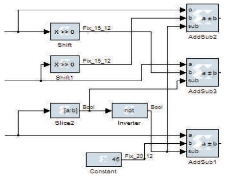
Figure 5. Iterative CORDIC Structure

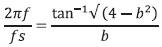
CORDIC has two operating modes, Vectoring mode and Rotation mode. This model uses the vectoring mode, and the equations used for the iterations are given in Eq. (4)( Ray Andraka, Jan-1998).

 

(4)

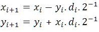
where
d_i = +1 if y₁ < 0,-1 otherwise
Then:

 

The decision function, d_i, is driven by the sign of the y or z register depending on whether it is operated in rotation or vectoring mode. In operation, the initial values are loaded via multiplexers into the x, y and z registers. During each of the next n clock cycles, the values from the registers are passed through the shifters and adder-subtractors and the results placed back in the registers. The shifters are modified to cause the desired shift in each iteration. Likewise, the ROM address is incremented in each iteration so that the appropriate elementary angle value is presented to the adder-subtractor. During the last iteration, the results are read directly from the addersubtractors. Obviously, a simple state machine is required to keep track of the current iteration, and to select the degree of shift and ROM address for each iteration. Here z is the output frequency control parameter which is fed from the accumulator output. As in the LUT based DDS, output frequency in CORDIC based DDS is also dependent on the reference-clock frequency (f_clk), Frequency Control Word (M) and length of N-bit accumulator. The resolution of the output waveform is dependent on the number of iterations. The CORDIC based DDS model is shown in Figure 6(a) and result is shown in Figure 6(b). Input clock frequency is 100 MHz, whole bit length is 9-bits and step size is 5.623. The output frequency is 1.11 MHz.

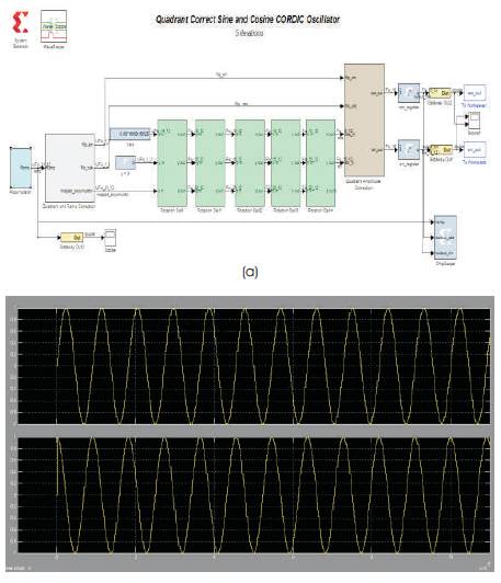
Figure 6. (a) Model of DDS using CORDIC algorithm (b) Output of the CORDIC based DDS model

The authors can also generate sine waves using marginally stable IIR filters. Consider the Simulink model of a simple two weight IIR (all-pole) filter shown in Figure 7.

Figure 7. An Infinite Impulse Response (IIR) filter as a sine wave oscillator

The output frequency (f) in this design is dependent on input reference clock frequency (f_s) and the value of 'b'.

From the equation below, we can calculate the output frequency by providing an input clock frequency and a constant value for b.

 

Here, the input clock frequency is 100 MHz and value of b is 1.75. The output frequency is 8.04MHz. Result is shown in Figure 8.

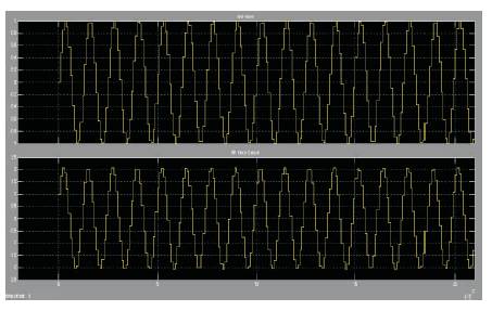
Figure 8. Output waveform of IIR filter used as sine wave generator

The authors discussed three different DDS architectures in this paper. They also now compare the different architectures with regard to the parameter of Spurious Free Dynamic Range (SFDR) value. SFDR will give the spectral purity of the output signal of DDS. Amplitude of the harmonics produced by any DDS system is dependent on the ratio of the output frequency to the input clock frequency. This is because the spectral content of quantization noise changes as the ratio changes, though its theoretical rms value is equal to (where q is the number of the LSB) (Vankka, J. 2001). The assumption that the quantization noise appears as white noise and is spread uniformly over the Nyquist bandwidth is simply not true in a DDS system. If the output frequency is an integral multiple of input clock frequency, then the quantization noise will occur at multiples of the output frequency. If the output frequency is slightly offset, then the quantization noise will become more random, thereby giving an improvement in the effective SFDR. Comparison of the parameters in different architectures is shown in Table 1.

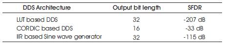
Table 1. Comparison of Different DDS Architectures

Having seen different designs of DDS, linear frequency modulated signal is now required to be generated. We can change any one of the three parameters to get a different frequency output. By varying a single variable repeatedly, we can generate a frequency modulated signal as desired.

In this paper, chirp signal is generated by varying the control word for the Phase Accumulator (PA) block. An increasing ramp output is given as input step word to the phase accumulator. By continuously varying the control word, there will be variation in the output frequency generated by the model as shown in Figure. 9. The input clock frequency is 320 MHz, step size in ramp generation block is 0.01 and 8 whole bits and 6 fractional bits are used in this model. We can also vary the start frequency by giving the start word in the second constant block present in the model. The output frequency will be varied till half of its input frequency obeying the Nyquist criterion. When using all the bits in phase accumulator, complete chirp will be generated and frequency generated will be half the input clock frequency, which is from 0 Hz to 160 MHz as shown in Figure 10(b). The BW of the system can also be decided by considering only the MSB bits and truncating the LSB bits coming from the word generator and thus generalize the system for any of the specified applications. In Micro-SAR, bandwidth required is 80 MHz, and therefore, 6 MSB bits are used as input to phase accumulator. Bandwidth of the generated chirp signal is 80 MHz as shown in Figure 11(b). Table 2 gives the specifications of the output signal generated with different MSB bit length.

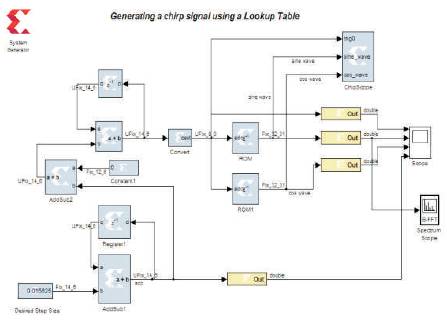
Figure 9. Chirp generator using LUT based DDS

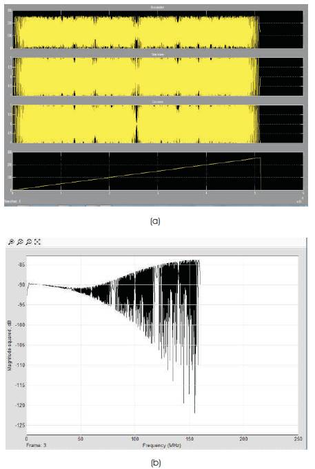
Figure 10(a). Chirp signal output of 8-bit input to PA (b) Spectrum of output frequency generated

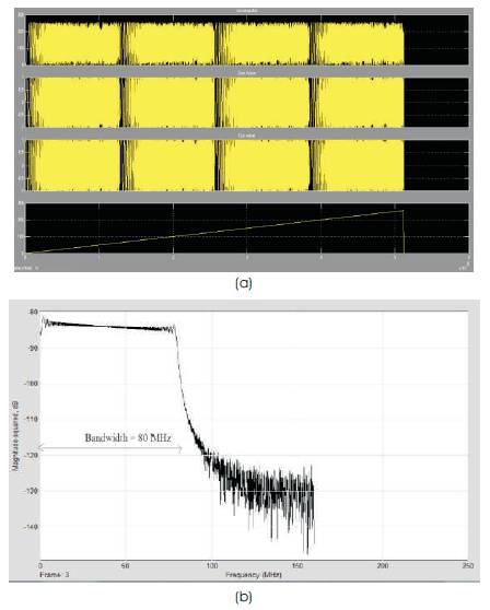
Figure 11. (a) Chirp signal output of 6-bit input to PA (b) Spectrum of output frequency generated

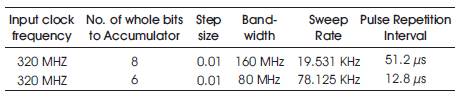
Table 2. Chirp Signal Output Specifications

Simulink model is used to generate a VHDL code which is synthesized and implemented in FPGA. Using the Chipscope Pro block, the output generated on the FPGA can be viewed. The board used for implementation is SPARTAN 3AN-XCS3AN700 starter kit board. Chirp signal output implemented in FPGA is shown in Figure 12. μSAR specifications are mentioned in Table 3 (Duersch M. I., Dec-2004).

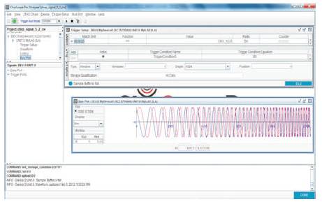
Figure 12. Chip Scope Pro output

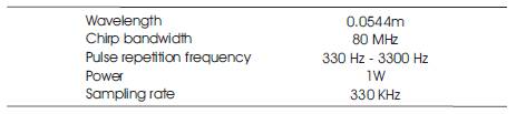
Table 3. μ SAR Specifications

LFM-CW waveform based μSAR provides a light weight, low cost and low power alternative to traditional pulsed radar systems, especially for highly constrained environments such as that obtained in UAV. In this paper, waveform generation using DDS has been implemented on FPGA. Different DDS architectures based on LUT, CORDIC and IIR have been simulated using System Generator blocks of Simulink. On comparison of the above methods based on parameters of SFDR and output bit length, it is deduced that LUT based DDS offers greater spectral purity than the other methods. Chirp signal with a bandwidth of 80 MHz has been generated according to the specifications of μSAR given in Table 3, using the technique of LUT based DDS. This chirp signal can be further used in many other radar applications.