Numerical simulations- i.e. the use of computers to solve problems by simulating theoretical models- is part of new technology that has taken place alongside pure theory and experiment during the last few decades. Numerical simulations permit one to solve problems that may be inaccessible to direct experimental study or too complex for theoretical analysis. Computer simulations can bridge the gap between analysis and experiment. Numerical simulations analysis and experiment cover mutual weakness of both experiment and theory. These simulations will remain a third dimension in ultrasonic measurements, of equal status and importance to experiment and analysis. It has taken a permanent place in all aspects of ultrasonic measurements from basic research to engineering design. The computer experiment is a new and potentially powerful tool. By combining conventional theor y, experiment and computer simulation, one can discover new and unsolved aspects of natural process. These aspects could often neither have been understood nor revealed by analysis or experiments alone. There might be many use of ultrasound but a common one is its application to nondestructive evaluation. Pulsed ultrasonic is finding an increasing number of applications in research and industrial non-destructive testing. In such evaluation, one tries to obtain information about the inner parts of an ensemble without dismantling it. In an ultrasonic system, a transducer consists of a collection of material layers. The design and optimization of a multilayered transducer is a complicated engineering task that involves knowledge of physical acoustics, analog electronics, and the acoustical properties of the materials involved. This task is made even more difficult by the lack of available information about frequency and thermal dependencies of these materials characteristics. The optimal combination of suitable materials can be found by trial and error, but not without considerable time and cost, both of which can be minimized through the use of simulations. The aim of this paper is to present a tool which provides a simulation of the received signal prior to construction. Of the different ways to model the electroacoustic system, a total electrical simulation tool is used for the following reasons. First, the modelling of acoustic wave propagation in one dimension by electrical lines can be handled with a certain ease; second the associated electronics used to excite, receive, amplify and process the signals can be designed to meet the application's specifications prior to building system. This paper presents a simulation solution to ease the selection process. The electronic software simulation package used is PSPICE [15]. The use of PSPICE provides an opportunity to simulate the complex set of excitation electronics, the ultrasonic transducer, the material under investigation, and the receiving electronics. Electrical analogies of one-dimensional acoustic phenomenon have studied over the years. Mason (1942) [23], modelled electromechanical transducers with a lumped equivalent circuit. Redwood (1961) [11], [17], simulated Redwood's implementation of Mason's model. Krimholtz et al (1970) [16], presented another equivalent circuit for elementary piezoelectric transducer. Leach (1994) [22], used controlled current and voltage sources instead of transformers. Leach mathematically derives his model by adding terms equal to zero in one of the devices electromechanical equations to obtain the form of the telegraphist's equation. Puttmer et al (1996) [3], used a lossy transmission line in Leach's model to account for acoustical attenuation. Benny et al (2000) [4], outlines a method that has been implemented to predict and measure the acoustic radiation generated by ultrasonic transducers operating into air in continuous wave mode. A comparison of experimental and simulated results for piezoelectric composite, piezoelectric polymer, and electrostatic transducers is then presented to demonstrate some quite different airborne ultrasonic beam-profile characteristics. San Emeterio et al (2004) [19], present an approximate frequency domain electroacoustic model for pulsed piezoelectric ultrasonic transmitters by which, integrating partial models of the different stages, allows the computation of the emission transfer function and output force temporal waveform. Song Hi Lee (2004) [21], obtained Shear Viscosity of some organic materials by Non-equilibrium Molecular dynamics Simulations, Hirsekon et al (2004) [13], perform numerical simulations of acoustic wave propagation through sonic crystals consisting of local resonators using the local interaction simulation approach (LISA). Ali (2000) [12] perform the simulations of a discrete time model of the impulse response of matched and backed piezoelectric transducers have been used to design sensitive short-response transducers Xiaoqi Bao et al (2003) [26] described a simulation and analytical models for the ultrasonic/sonic drill/corer (USDC) . Aouzale et al (2009) [27],. simulate the diffraction losses in a pulse-echo ultrasonic system. Diana Engelke et al (2011) [28], demonstrates the benefits to simulate an ultrasonic dental scaler by means of the FEM. Existing methods for the modeling of piezoelectric transducer response are generally frequency domain-based. The major disadvantage of this type of model is that they cannot take into account the electrical elements present in the emitting or receiving circuit whose values vary with respect to time. The need for a method that accounts for time-varying elements arises, for example, when the circuit comprises active electrical elements, such as diodes, or when the transducer is excited by capacitive discharge via a switch. A time domain-based method is presented by Sferruzza et al (2002) [20], to compute the electro-acoustical response of a piezoelectric transducer and its electrical circuit, taking into account in the presence of time-varying elements.

The current work applies the approach of Puttmer et al [3] to liquids and piezoelectric transducer to obtain an electrical analogue of one-dimensional, acoustic wave propagation through such materials. In order to keep things at a manageable level, the following simplifications and assumptions are made. The acoustic propagation travels along one direction and consist of planner longitudinal waves, which are normal to the direction of propagation. The amplitudes are small enough to keep things in linear regions of the devices such that the principle of superposition is not violated. From available material data, such as the modulus of elasticity and Poisson's ratio, the necessary electrical parameters are deduced. Validation of the theory is achieved by comparing experimental data obtained from different liquids at fixed frequency and temperature.

System Modeling

The piezoelectric phenomenon is modelled using controlled voltage and current sources [22] [Figure 1].

Here l is the thickness, f is the force, u is the particle velocity, v is the electrical voltage, i is the electrical current, h is the piezoelectric constant and s is the Laplace operator.

The equivalent circuit consists of the static capacitance C0 (capacitance between the electrodes), a transmission line (representing the mechanical part of the piezoelectric transducer) and two controlled sources for coupling between the electrical and mechanical part of the circuit. Suppose a ultrasonic pulse travels through a medium with a finite speed c (m/s). This pulse can be pictured as a disturbance to which the medium reacts to. In the case of longitudinal wave, the disturbance is a compression or rarefaction of matter, which the medium displaces to return to its equilibrium state. The compression and rarefaction within the medium is related to its density ρ (kg/m³), and the restoring force is related to the medium's bulk modulus M (pa) [10]. Their relationship to the speed of sound is:

c = v M/ρ.

Similarly, in an electrical transmission line an electrical pulse can travel through it. These pulses are received at the other end of the line after a very short but finite time. The pulses travel at a certain velocity. Similar to the acoustic wave, the electrical pulses are concentrations and rarefaction of electrons within the transmission line [8].

A distributed-parameter network with the circuit parameters distributed throughout the line can approximate a lossy transmission line. One line segment with the length Δx can be approximated with an electric circuit as in the following Figure 2.

This lossy transmission line model is described by four lumped parameters,

• R is the resistance in both conductors per unit length in Ω /m
• L is the inductance in both conductors per unit length in H/m
• G is the conductance of the dielectric media per unit length in S/m
• C is the capacitance between the conductors per unit length in F/m

Where R and G is zero under lossless conditions.

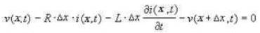
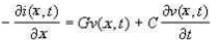
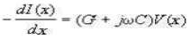
To derive the parameters the authors begin by using Kirchhoff´s voltage law on the circuit in Figure 1.

(1)

which can be written as:

(2)

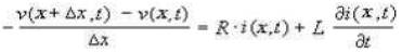
and then letting Δ x→0 we get:

(3)

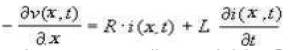
Then they have one equation containing R and L. To get another equation relating G and C, here they apply Kirchhoff´s current law on the circuit and get:

(4)

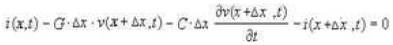
and letting Δ x→0 in this equation also we get

(5)

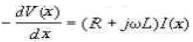
The first order partial differential equations, equation 3 and equation 5, are called the general transmission line equations. These equations can be simplified if the voltage v(z,t) and the current i(z,t) are time-harmonic cosine functions:

(6)

(7)

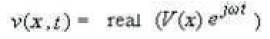
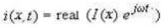
Where ω is the angular frequency. Using equation (6) and equation (7), the general transmission line equations in equation (3) and equation (4) can be written as:

(8)

(9)

These equations are called the time-harmonic transmission line equations. These equations (equation (8) and equation (9)) can be used to derive the propagation constant and the characteristic impedance of the line. By differentiating equation (8) and equation (9) with respect to z, hence,

(10)

(11)

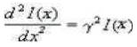
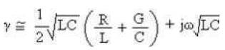
Where γ is the propagation constant:

(12)

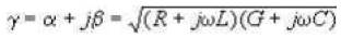
The real part α, of the propagation constant is called the attenuation constant in Np/m and the imaginary part, β, is called the phase constant of the line in rad/m. The general solution to the differential equation (10) is

(13)

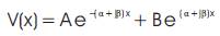
The time dependence into the equation (13) can be obtained by multiplying e^jωt to equation (13).

(14)

Equation (14) describes two travelling waves; one travelling in the positive x direction with an amplitude A which decays at a rate α while the other with an amplitude B travels in the opposite direction with the same rate of decay.

The same type of differential equations governs the propagation of an acoustical wave. In the case of harmonic waves, corresponding to equations (10) and (11), we have the lossy linearized acoustic plane wave equations.

(15)

(16)

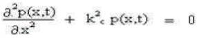
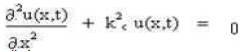
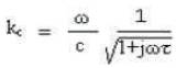
where p(x, t) (Pa) is the pressure and u(x, t) (m/s) is the particle velocity [10]. Equivalent to γ, kc is the complex wave number composed of an attenuation constant a (Np/m) and a wave number k (rad/m). The general solution of the wave equation (15) is,

(17)

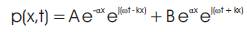
and is identical to the solutions obtained in transmission line's represented by equation (14). Equation (16) has a solution of the same form. The complex wave number k_c is given as

(18)

Where τ is the relaxation time [10].

Using equations (17) and (18), we get

(19)

and

(20)

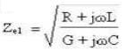
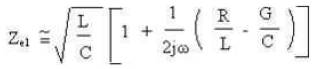
In order to unify the two theories, an impedance type analogy is chosen where mechanical force is represented by voltage and current represents particle velocity. The characteristic impedance becomes important at the boundaries because there the continuity conditions have to be satisfied. Pressure and normal particle velocity must be continuous at the boundaries as voltage and current must be continuous at connections. For the lossy transmission line [8], the characteristic impedance Z_e1 is:

(21)

and for the lossy acoustic medium [10] ,the characteristic acoustic impedance Za is:

(22)

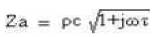
where ρ is the density of the medium.

Expanding equation ( 21) and equation (12), we obtain,

(23)

And

(24)

Considering small but non-negligible losses where R << ωL, G << ωC and ωτ << 1. the second term of equation (23) is negligible, leaving the characteristic impedance as . Similarly from equation (22), the low loss acoustical characteristic impedance can be approximated as ρc. Also, the wave number k from equation (20) become ω/c. To correlate the two characteristic impedances, we choose an impedance type analogy (Figure 1), in which the force, (and not pressure) is represented by voltage and the particle velocity is represented by current. The equivalence between the two systems is

(25)

where A (m2) is the cross-sectional area of the acoustic beam.

Assisted with the definition of the low loss characteristic impedances equation, following relationships can be obtained

(26)

(27)

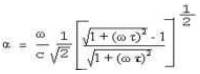
The real part of equation (24) is the attenuation constant

(28)

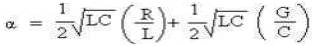
Drawing a parallel with the classical theory of acoustic attenuation,

α_classical = α_v + α_tc

where α_v is the coefficient of attenuation due to viscous losses, and α_tc is the coefficient of attenuation due to thermal conduction. From equations (26), (27) and (28), we can solve for R and G to model the attenuations such that,

(29)

(30)

Because the material layers used in this paper have a low heat conductance, the loss due to thermal conduction is negligible, and we let the conductance G = 0.

Equations (26), (27), and (29) are the final equations required for simulation purpose.

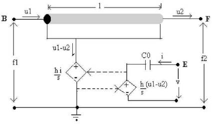
Figure 1. Equivalent circuit for piezoelectric transducer (The Leach model)

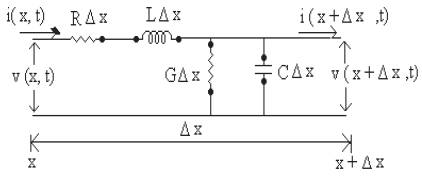
Figure 2. Equivalent circuit of an element of a transmission line with a length of Δx

An important task when designing ultrasonic transducers and complete transducer system is the simulation of possible configuration prior to construction. Ultrasonic transducer usually consists of a piezoelectric element and non-piezoelectric layers for encapsulation and acoustic matching. Points of interest are effects of backing materials, matching layers, piezoelectric materials, layer thickness, electrical matching and coupling on transducer characteristics like bandwidth, time response on different excitation signals and ring down behavior. As presented in the introduction, different models have been developed over the years to simulate these transducers. Mechanically, a transmission line T of length len (m) represents the acoustical layer. The length is selected to achieve the desired center frequency f (Hz) of the transducer. With fixed ends, the piezoelectric plate has a fundamental resonant frequency as:

(31)

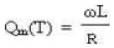
Where c (T) is the velocity of sound through it at temperature T. Using equations (26), (27) and the piezoceramic's density ρ, required for transmission line, L and C values can be calculated. The mechanical factor Qm describes the shape of the resonance peak in the frequency domain. The relation between angular frequency ω, inductance L and the resistance R is given as [3]

(32)

In the electrical section, the static capacitance Co is calculated as :

(33)

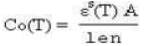
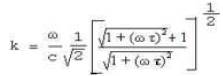
where ε^s (C² /Nm² ) is the permittivity with constant strain [9]. The latter is related to the permittivity with constant stress (free) ε^T as

(34)

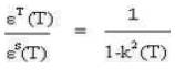
Where k (T) is the piezoelectric coupling constant.

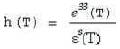
The mechanical and electrical sections interact with two current controlled sources. From the mechanical side, the deformation itself is not measurable, but the current representing the rate of deformation is the difference between the velocity of each surface normal to the propagation path, represented by the currents u₁ and u₂ ,  is the rate of deformation. This current (u₁ - u₂ ) controls the  current source F₁ . It has a gain equal to the product of the  transmitting constant h (N/C), and the capacitance C₀. h  is the ratio of the piezoelectric stress constant e³³ (C/m² ) in the direction of propagation and the permittivity with zero  or constant strain ε^s . In the thickness mode it is [9].

(35)

This source's output is in parallel with the capacitor Co. The result is a potential difference across the capacitor that is proportional to the deformation. In the electrical section, the current through the capacitor Co controls the current source F2. The gain for this second current source is h. Its output needs to be integrated to obtain the total charge on the electrodes that proportionally deforms the transducer. The integration is performed by the capacitor C₁ . The voltage controlled voltage source E₁ with unity  gain is a one-way isolation for the integrator.

The speed of sound in a liquid is given as:

 

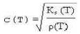
Where Ks is the adiabatic bulk modulus [2].

Starting with the Navier-Stokes equation, Kinsler et al [10] derive the following formula for the coefficient of attenuation due to viscosity

 

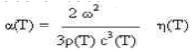
Where η(T) is the viscosity of liquid. One of the assumptions made in this derivation is that the bulk viscosity is negligible. Parameters that are temperature sensitive, like viscosity, need to be obtained at the desired temperature for single temperature simulation or as a function of temperature for parametric simulation over a temperature range.

Experimental Setup

The block diagram of pulser-Receiver system is shown in Figure 3. The experimental circuit is designed by Gandole et al [18] is used in this set up. The RF pulse generator generates sharp radio frequency pulses of various frequencies in the range 1 MHz to 10MHz, having pulse width 2 to 60 microseconds. The repetition rate of the pulses is 1 KHz. The radio frequency pulse is fed to the ultrasonic transducer (piezoelectric). The transducer excited and sends ultrasonic pulse through the sample. The receiver transducer, which is at the other end of the sample, converts the received ultrasonic pulse into an electrical signal (RF pulse). The details of pulser circuit are given in Gandole et al [18]. This RF pulse is fed to an amplifier consists of single stage which is assembled by using transistor BF195. The output of single stage amplifier is again amplified with the help of another amplifier using IC CA3028 in cascade mode. The overall characteristics of amplifier are as: gain = 50 dB; bandwidth = 15 MHz; input impedance = 10.5 kΩ and low noise. The stability of IC 3028 amplifier is much higher because of small reverse feedback [14]. After the detection of signal through LM 393 (wide band zero cross detector), the detected signal is fed to unity gain buffer, designed using high speed, low power Op-amp AD 826. The characteristics of AD826 are 50 MHz unity gain bandwidth, 350 V/μs slew rate, 70 ns settling time to 0.01% and 2.0 mV max input offset voltage. This detected signal is then given to reset input of RS flip-flop, while the output of IC 74121 of RF pulse generator is used to set the flip-flop. Therefore a single pulse is obtained at the output, whose width is the time taken by the pulse to travel through the sample. Time meter having accuracy of 0.01 μs measures the width of the pulse. For the measurement of velocity and attenuation, the sender transducer is firmly fixed at one end of the measuring cell (Figure 4), while receiving transducer is fixed to movable scale (Griffin and Tatlock Ltd. London, Make) having least count 0.0001 cm. The system communicates with personal computer (PC) through 12-bit DAS card. For communication, control and set of parameters of ultrasonic system Graphical user interface (GUI) were created (Figure 5). GUI provides general data representation. In GUI it is possible to change almost all of parameters of measured signal and parameters of signal processing. For link-up with system functions for control drivers in Dynalog system were used. Then parameters for communication with system were set up. In windows (Figure 5), it is possible to select channel number, polarity (unipolar/Bipolar) and Range using DAQ configuration frame. “RUN DAQ” frame is used to open the card using “open” command button, close the card using “close” command button. “Start Scan” command button samples the data (voltage level and time) and stores in buffer memory. “Stop Scan” command button stop the sampling process. Measurement and analysis of received ultrasonic signal is achieved by “Measurement and Analysis” frame. The command button “Transient Response” opens the new window, which displays the transient response of the sampled data. Using the cursor point it is possible to measure the time and pulse height of received signal. This data is stored in database for further analysis. Matched pair of quartz transducers completely sealed (supplied by electrosonic industries, New Delhi.) was used for ultrasonic generation and detection. The frequency of measurement was 2 MHz. Diameter of transducer was 25.4mm. Also the second set of matched pair of transducer PZT-5A (supplied by Panametrics Videoscan V3456) with centre frequency 5 MHz was used. Diameter of transducer was 12.5 mm. The liquid sample was contained in a measurement cell as shown in Figure 3. A glass bottle of suitable size was cut to form a measuring cell. The bottle was fixed with adhesive araldite in an inner space of double walled chamber which was made up of thick galvanized sheet. Water circulation arrangement was made through thermostat. Dimensions of double walled chamber are as: height of doubled walled chamber 6.5 inches, outer diameter 5.5 inches, inner diameter 3.25 inches, height of glass bottle 7.5 inches. The double walled chamber was provided with inlet and outlet for constant temperature water circulation. The lower surface of cell (glass bottle) and double walled chamber were in the same plane. The double walled chamber was kept on disc to which sender transducer was fixed. Applying silicone grease made the contact of sender transducer and measuring cell. The lower surface of measuring cell acted as acoustic window through which ultrasonic waves could enter in the measuring cell. The clamps were provided between double walled chamber and disc to avoid movement of doubled walled chamber and hence of measuring cell during the ultrasonic measurements.

The analogous circuit setup is described in Figure 6. Simulation code is given below, to describe the circuit.

Here Static capacitance (Co)=C₁ =C₄ , R₁ =R₅ , F₁ =F₃ , F₂ =F₄ , E₁ =E₂ .

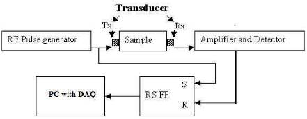
Figure 3. Block diagram of experimental setup

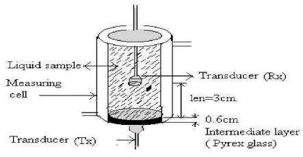
Figure 4. Probe layout for liquid samples

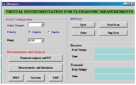
Figure 5. GUI Screen of Experimental ultrasonic system Simulation Setup

The Pulser-receiver

The pulser circuitry, shown in Figure 6 consists of a pulse generator using pulse source (V₂ ) having 5V pulsed  voltage, 0 sec delay, 1ns rise and fall time, 2us pulse width and 1ms period. Another source (V₃ ) is sinusoidal source having 0 offset voltage, 5V peak voltage, 0 sec delay, 5MHz frequency, 0 damping factor and phase delay followed by TTL7400, 7407, 1KΩ resistor (R₃ ), 20V dc supply  (V₁ ) and 2nf capacitor (C₃ ). The pulse start at 20 V and  decays to 0 V in 2us. The output of the capacitor is connected to the electrical part of the transducer and a parallel damping resistor (R₄ ). The receiving and amplifying  electronics is not implemented in this schematic.

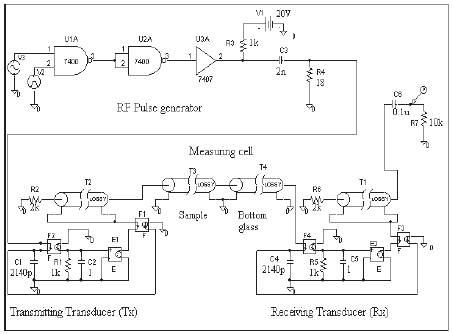
Figure 6. Simulation circuit of the experimental setup

The Transducer and liquid Samples

The matched pair of piezoelectric material PZT-5A, whose material data is obtained from Berlincourt [5], was chosen and given in Table 1. For simplicity, the front wear plate is omitted, and to reduce the ringing of the echoes a backing material is selected with a characteristic acoustic impedance of 15.8 MPas/m. The thickness of the backing layer should be selected such that no echoes return from it. This facts permits us to model the backing layer with a resistor (R₂ = R₆=2KΩ). Another matched pair of quartz transducers supplied by electro sonic industries, New Delhi, was chosen and whose material data is given in Table 1.

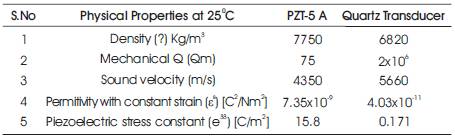
Table 1. Physical properties of materials at 25^o C

Graphical User Interface for Simulation Analysis

Figure 7 shows the Graphical User Interface (“UT Measurements”) for easy access to the basic functionality of the modeled ultrasonic system using PSPICEA_D. The results of mixed-signal simulations can then be plotted in the same Probe window with little effort. The newly developed Graphical User Interface heightens the level of clarity, accelerates the speed of navigation and improves control of information flow enabling end users to take advantage of the systems full potential.

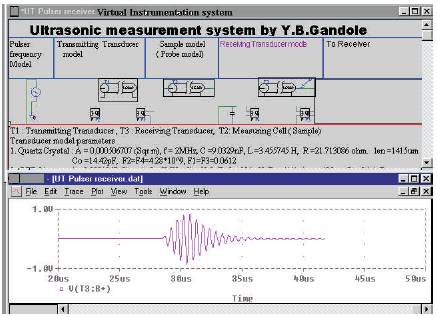
Figure 7. GUI Screen for modeling and simulation of ultrasonic system

Signal Processing

1. Time Domain Analysis

Comparing the received signals from experiments and simulations in the time domain. The simulation signal is shown in (a) and the measured signal is shown in (b). Figure 8 shows the first 30 us pulse received by the 5 MHz  transducer with an ethanol sample at 25^o C.

Figure 9 shows the first 32 us pulse received by the 5 MHz transducer in Methanol at 25^o C.

Figure 10 shows the first 36 us pulse received by the 5 MHz  transducer in Carbon tetra chloride at 25^o C.

Figure 11 shows the first 30 us pulse received by the 5 MHz  transducer in Acetone at 25^o C.

Figure 12 shows the first 27 us pulse received by the 5 MHz  transducer in benzene at 25^o C.

Figure 13 shows the first 25 us pulse received by the 5 MHz transducer with a distilled water sample at 25^o C.

Table 2 shows the comparison between the literature values and simulation values of ultrasonic velocity and attenuation for the liquid samples.

Figure 14 (a-e) shows the first 50 us pulse received by the 2 MHz crystal transducer with binary liquid mixtures of Methanol and benzene sample at 25^o C.

Figure 15 (a-e) shows the first 50 us pulse received by the 2 MHz crystal transducer with binary liquid mixtures of Methanol and benzene sample at 25^o C.

Table 3 (a-b) shows the comparison between the Experimental values and simulation values of ultrasonic velocity and attenuation for the binary liquid mixture samples.

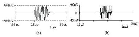
Figure 8. Complete transient received by 0 5MHz transducer at 25^o C, in Ethanol

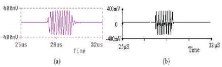
Figure 9. Complete transient received by  5MHz transducer at 25^o C, in Methanol

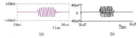
Figure 10. Complete transient received by 5MHz transducer at 25^o C, in Carbon tetra chloride

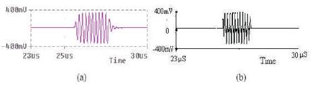
Figure 11. Complete transient received by  5MHz transducer at 25^o C, in Acetone

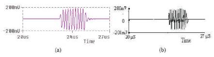
Figure 12. Complete transient received by  5MHz transducer at 25^o C, in Benzene

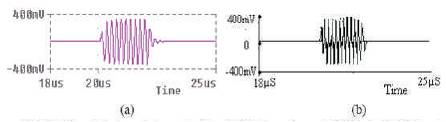
Figure 13. Complete transient received by  5MHz transducer at 25^o C, in distilled water

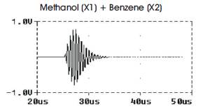
Figure 14 (a). Methanol + Benzene Mole fraction X1=0.1952

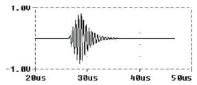
Figure 14 (b). Methanol + benzene Mole fraction X1=0.4834

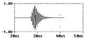
Figure 14 (c). Methanol + benzene Mole fraction X1=0.6858

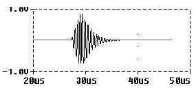
Figure 14 (d). Methanol + benzene Mole fraction X1=0.8359

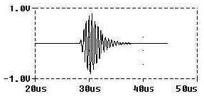
Figure 14 (e). Methanol + benzene Mole fraction X1=0.9516

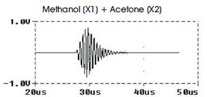
Figure 15 (a). Methanol + Acetone Mole fraction X1=0.1678

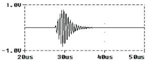
Figure 15 (b). Methanol + Acetone Mole fraction X1=0.4375

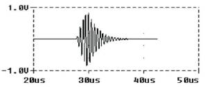
Figure 15 (c). Methanol + Acetone Mole fraction X1=0.6447

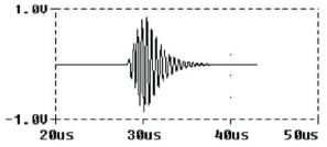
Figure 15 (d). Methanol + Acetone Mole fraction X1=0.8090

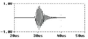
Figure 15 (e). Methanol + Acetone Mole fraction X1=0.8090

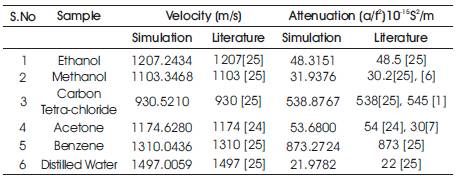
Table 2. Ultrasonic velocity and attenuation at 25^o C for 5 MHZ frequency

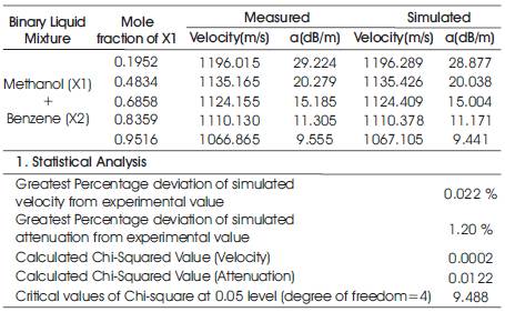
Table 3 (a). Comparison of measured and simulated values of ultrasonic velocities and attenuations in binary liquid mixtures (Methanol and Benzene) at 25^o C

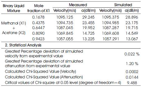
Table 3 (b). Comparison of measured and simulated values of ultrasonic velocities and attenuations in binary liquid mixtures (Methanol and Acetone) at 25^o C

Analogy between acoustic media and transmission lines is reviewed and an analogous electrical model of an ultrasonic transducer using controlled sources is discussed. A simulation model of a complete ultrasonic system is presented. The received signal from the simulation is compared to that of an actual measurement in the time domain. The comparison of simulated, experimental data clearly shows that temperature and frequency dependencies of parameters of relevance to acoustic wave propagation can be modelled. The feasibility has been demonstrated in an ultrasound transducer setup for material property investigations. Comparisons were made for attenuation and velocity of sound for ethanol, methanol, carbon tetrachloride, acetone, benzene and distilled water. For these materials, the agreement is good. The simulation tool therefore provides a way to predict the received signal before anything is built. Furthermore, the use of an ultrasonic simulation package allows for the development of the associated electronics to amplify and process the received ultrasonic signals.