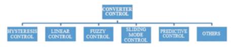
Figure 1. Basic Methods of Converter Control
This paper traces the basic concepts behind the predictive control strategy used in power converters and drives. Wide research on predictive control has been increasing day-by-day. With the availability of new digital control techniques, various schemes has been proposed. Predictive control scheme presents several advantages over other control schemes that makes it capable for various applications in the field of power electronics and drives i.e. inclusion of constraints and nonlinearities. A classification of predictive control scheme is presented and each scheme is described along with its application. This paper reflects the robustness as well as flexibility of predictive control scheme. Predictive control scheme has the capability to advance the performance of future energy processing and control systems.
Power converters are used in various sectors ranging from industrial to domestic applications [1, 2]. Since, last 20 years, the control of power electronics and drives had become very important topic in order to increase the energy demands as well as the efficiency of the system. Various control techniques had been proposed for the control of power converters and drives. Some of them are shown in Figure1.
Figure 1. Basic Methods of Converter Control
They are hysteresis, linear control, fuzzy, sliding mode control, predictive control, adaptive control and many other techniques. Hysteresis and linear control techniques were the oldest among all[3-5]. In linear control scheme, there exists a problem of cascaded structure. Later on with the availability of new digital control techniques and inexpensive microcomputers, the new control techniques are implemented. Some of them are fuzzy logic, sliding mode control, adaptive control and predictive control. But amongst all the schemes, the predictive control is considered best to control the power converters. The drawbacks of various other control strategies are as follows:
All these problems were resolved in predictive control scheme thus obtaining a very fast transient response. Also the resulting controller is easy to implement. Predictive control for power electronics has been presented since 1980's. It has been applied to various converter and drive applications [6], in a three- phase inverter [7-10], and a matrix converter [11].
The paper is organized as follows: Section 1 presents the general concept of predictive control scheme along with its classification. In Sections 2,3,4 and 5, the structure of various predictive control schemes has been explained along with some application examples.
The first idea for predictive control methods has been published in 1960s by Emeljanov. The predictive control is considered as any algorithm that uses a model of the system for the future behavior prediction of the control variables which results in the sequence of control signals. The most appropriate control action is selected based on optimality criterion. In this algorithm, model of the process and the scenario for the future control signals are assumed. Predictive control schemes are mainly categorized into four types: hysteresis, trajectory, deadbeat and model based predictive control (continuous and finite set MPC) as shown in Figure 2. The functional principle of all these schemes are different based on different optimization criterion.
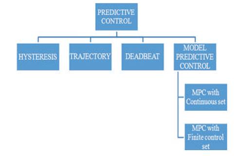
Figure 2. Classification of Predictive Control Method
For hysteresis based scheme, the criterion is to keep the controlled variables within the hysteresis area boundary. While in trajectory based predictive control the optimization criterion is to force the variables to follow a predefined trajectory. In case of deadbeat control, the optimal actuation is to make the error equal to zero in the next sampling instant. The criterion of model based predictive control is to minimize a cost function. The deadbeat control and MPC (with continuous control set) require modulator to generate the required voltage which results in a fixed switching frequency while other controllers doesn't require any modulator, thus provides a variable switching frequency.
The basic principle behind this type of control scheme is to keep the values of controlled variable within the tolerance band known as hysteresis area or space. “Bang-Bang controller” is the simplest form of this type of scheme. An improved form of a bang-bang controller is the predictive current control scheme proposed by Holtz and Stadfeld [12]. By the use of this controller, the switching instants are determined by the limits of tolerance band.
Figures 3 and 4 shows the functional principle of hysteresis based predictive control. Here, a circular boundary is chosen whose location is controlled by the stator current reference vector is*. If the actual value of current vector reaches the circular boundary line, then the next switching state vector is selected by prediction and optimization. Firstly, the future trajectories of the stator current (for all possible switching instants) are computed and then the time instants are determined required to reach the error boundary again. The circular tolerance region is itself moving in the complex plane along the stator current space vector. This movement is indicated by the dotted circle in Figure 4.
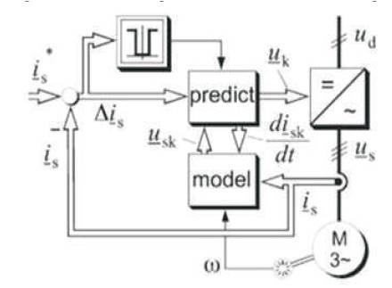
Figure 3. Hysteresis Based Predictive Control
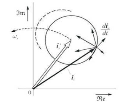
Figure 4. Predictive Current Control, Boundary Circle, and Space Vector
The predictions of switching instants are the well known mathematical differential equations of electric machines. Finally, the switching state vector possessing the longest stay-time within the hysteresis is selected and thus the switching frequency is minimized. Also other optimization criteria are possible like minimum current distortion or minimum torque ripple.
The advantage of this type of control strategy is that it does not require the specific knowledge of the system to be controlled. The hysteresis controllers are used to keep the control error within the specific limit band. But it must be ensured that hysteresis controller should react quickly if actual value will go outside the band. So, this is the major problem if it is implemented in a digital processor. Hence, hysteresis based predictive control is more suitable in case of analog operational amplifiers.
The basic principle of this type of control strategy is to force the system variables onto the precalculated trajectories. Once the system is forced onto one of these trajectories, it remains there until some change is done from outside. The first trajectory based control scheme was published in 1984 by Kennel[13]. According to this strategy, control algorithms were published like Direct Self Control (DSC) by Depenboock [14] or Direct Mean Torque Control by Flach [15].
Various schemes like sliding mode control [16] or DTC (Direct Torque Control) [17] are the combination of trajectory and hysteresis based predictive control strategies while DSPC by Mutschler [18] is considered as a trajectory based control scheme, but it contains few aspects of hysteresis based scheme also. In DSPC shown in Figure 5, there is no control loop to control the drive speed. So in order to control the speed directly the inverter switching events are calculated in a time-optimal manner.
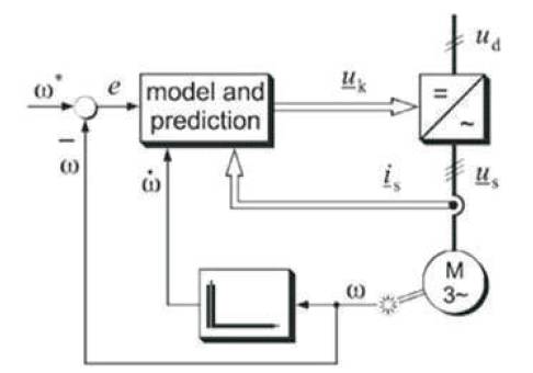
Figure 5. DSPC Block Diagram
The switching states of the inverter are divided into groups as torque increasing, slowly-torque decreasing, quicklytorque decreasing. For short time durations, the inertia as well as the derivatives of the load and machine torques is assumed as constant values. So, the system behavior is demonstrated by a set of parabolas in the speed error versus acceleration plane as shown in Figure 6. Here, initially the system state is assumed to be at point [ek ,ak ] T. The desired operating point is always the origin of the coordinate system i.e. zero acceleration as well as no error. But this condition does not exist for a long duration as infinite switching frequency will be required in this case. From –Hy to +Hy a kind of hysteresis band is defined in order to limit the maximum frequency to an acceptable value. Firstly, the torque increasing switching state Sk is chosen. The state starts moving along the dotted parabola until the new point [ek +1, ak +1]T is reached i.e. the point of intersection of the torque increasing parabola with another parabola for a torque decreasing switching state Sk+1. This parabola will pass through +Hy. The intersection point has been determined as the optimal time instant in order to reach the desired state point +Hy as fast as possible. Exactly in the precalculated time instant, the inverter is commutated into switching Sk+1. Now the system state is moving along the new parabola until the next point of intersection occurs when the torque decreasing parabola meets the torque increasing parabola i.e. at point [ek +2,ak +2]T is reached. At this point, a state Sk+2 (a torque increasing state) is chosen. Now the system state moves along the corresponding trajectory which is passing through -Hy until it reaches the parabola with state Sk+1. In steady state operation, the system state moves along the path (+Hy ) – [ek +2,ak +2]T – (-Hy) - [ek +3,ak +3]T – (+Hy ). Thus speed error i.e. e is kept in between the hysteresis band -Hy to +Hy . Hence, the speed is controlled directly without a cascaded structure.
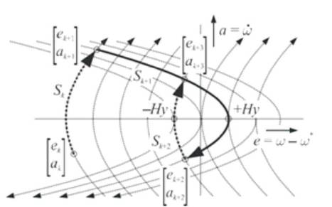
Figure 6. DSPC: Trajectories in the [e,a]T -state plane
Unlike hysteresis based predictive controllers, these type of controller requires an exact model of the system to be controlled. These are best suited for implementations in digital controllers on microprocessor.
The basic approach of deadbeat predictive control is to bring the output response to rest after a few finite time steps. This can be obtained by forcing the state vector to zero at time step h, i.e. x(t+h) = 0, h is called prediction horizon. A solution is given by the standard state feedback control law as follows,

where * denotes the pseudo inverse of the matrix. A and B are the matrices of the discrete time state space model of the system. Deadbeat predictive control can be accomplished through an input – output model.
Three deadbeat control algorithms were developed to compute the deadbeat predictive control law. These algorithms are simple and easy to implement. The first algorithm is designed based on indirect method, uses the multi-step-ahead output prediction to compute the control law. All calculations are performed recursively. The most difficult task is to calculate the pseudo inverse of a Hankel matrix formed by the system pulse response time history. Hankel matrix plays an important role in establishing the rule of selecting the identification parameter and the control design parameter i.e. control horizon. The second algorithm is based on direct method. It was developed by combining system identification and control law into one formulation. It directly computes the Hankel matrix and other quantities from input and output data. It is more efficient than the first type of algorithm. The third algorithm provides the state space representation of the deadbeat predictive control law. It computes the deadbeat gain for observer based full state feedback that may be converted into the input and output gain used in the classical predictive control designs.
Deadbeat predictive controller is a linear controller with feedback stabilization property. It can control time varying systems. But it has various disadvantages too like errors in the model parameter values, also non-linearities and constraints are difficult to apply in this case. Figure 7 shows the basic block diagram of deadbeat current control scheme [37]. Here modulator is used to generate the reference voltage.
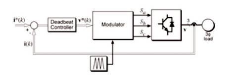
Figure 7. Deadbeat Current Control Scheme
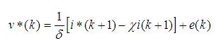
The load model for a RLE load in discrete time system is defined by the following equation:
Where
Figure 8 shows the basic operating principle of deadbeat current control. At time k, the error is generated due to load current i and reference current i*. This error is used to calculate the reference voltage v* which is applied to the load at time k. At time k+1, the load current will be equal to the reference current.
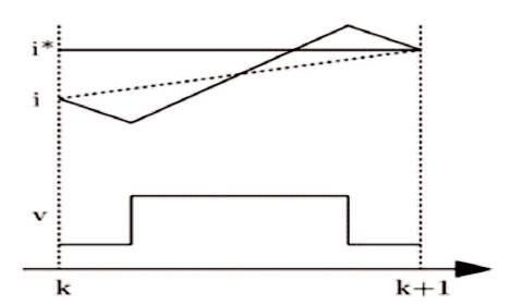
Figure 8. Illustration of Deadbeat Current Controller Operation
It is used for various applications like current control in three phase inverters [7, 19-28], rectifiers [29, 30], active filters [31, 32], uninterruptible power supply [33-35], DCDC converters [36].
Model Predictive Control (MPC) is a digital control strategy initially developed for oil and petrochemical industries, and later on its application area increased in power converters also. The MPC is also known as, “Receding horizon control approach” [37]. As compared to other conventional predictive control schemes, MPC is completely based on different ideas. The other predictive control schemes discussed use only the present value of the system to calculate the next switching instants while, MPC deals with the past as well as the present values of the system for the future prediction calculation. Also, MPC finds the best switching instant, not only for the next cycle but up to a specified horizon i.e. control horizon. Clarke [38] had described a Model based Predictive Control along with their historical development. He also proposed Generalized Predictive Control (GPC) as one of the model based predictive algorithm [39]. MPC is a multivariable control algorithm uses model of the system to predict the behavior of the variables until a certain horizon of time and a cost function is defined which represents the desired behavior of the system. The optimal actuation is obtained by minimizing the cost function.
Figure 9 illustrates the functional principle of the Model Predictive Control. The main central part of the system is the model. Using this model, the future behavior of the system is predicted over a time horizon. The prediction response mainly consists of two components: forced response and free response. Free response shows the expected behavior of the system output y(t+j) assuming future values of the actuating variables being equal to zero and forced response is the additional component based on the pre-calculated set of future actuating values u(t+j).
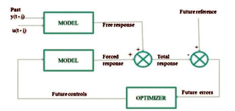
Figure 9. Block Diagram of MPC
For linear systems, the total response is equal to the summation of both the components. This sum is calculated up to the finite prediction horizon Np. The total response is compared with the future reference values generating future error. Then an appropriate control sequence u (t+j) is calculated in order to reduce the tracking error by minimizing a quadratic cost function as well as considering all the system constraints. This is done in an optimizer. A simple open-loop strategy would only apply this pre-calculated future sequence of values for the actuating variables of the system. The use of receding horizon approach change it into closed loop control by using past values of the output as well. Only the first element u(t) of the sequence is used while others are rejected and complete process of prediction, optimization and controlling is repeated at every sampling instant. Hence, the prediction horizon is shifted forward as shown in Figure 10.
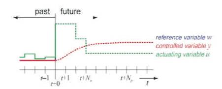
Figure 10. Definition of Control and Prediction Horizon
Control horizon is introduced in order to reduce the calculation complexity i.e. Nu. After Nu steps, it is assumed that the controller output helds constant.
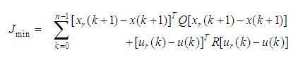
The cost function is defined by the following quadratic equation:
With the notation:
J = cost function
x = controlled variable,
u = manipulated variable,
n = prediction horizon,
Q, R is the weighting matrices used to weight prediction error and control actions.
Cost function consists of two parts:
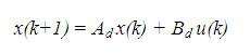
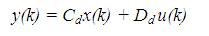
Along with the cost function, the model is the most important part of MPC. The dynamic model is used for MPC. Both continuous time and discrete time models may be used but only discrete is preferred since it is beneficial to consider the discrete nature of the controller in the first step of the controller design and hence to use a discrete-time system description.
It is the simplest form to get a discrete-time representation of the system. A linear system can be easily represented in a state space description in discrete – time domain as,
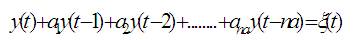
These models are based on the transfer function of the controlled system. It consists of various types of models.
This model can be expressed as follows:
or
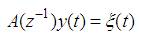
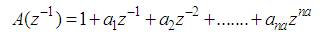
where
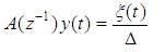
The function ξ(t) represents the noise and disturbance which is affecting the system.
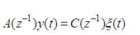
It is an extension of the AR model with an integrated noise term expressed as :
where, 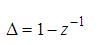
Therefore,
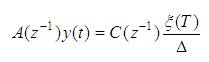
In this model, the noise is represented with an extended term:
In which,

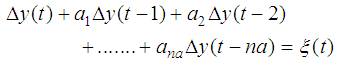
In this model also, noise is considered with an integrated structure. It is represented as follows,
It is almost similar to ARMA, but possesses additional input variables which represent the actuating variables from outside. It is represented as,
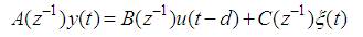
In which,
where, d represents the time delay or dead time between the input u and output y of the system. This model is also known as Controlled Auto Regressive Moving Average Model (CARMA).
This model is an extension of ARIMA model. Additional input variables are included here. It is represented as,
These models represent the behavior of a non linear control system. Amongst all the non linear models, Hammerstein and Wiener model are the most prominent ones. Besides these, there is another method of modeling non–linear systems with the NARMAX model. NARMAX stands for non linear auto regressive moving average model with eXogenous inputs that are described in detail by Leontaritis/Billings [40, 41].
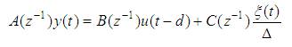
Model predictive control considers the inherent discrete nature of power converters along with the inclusion of constraints and nonlinearities. Power converters have finite number of switching states so the optimization problem is simplified and thus prediction is done only for those possible switching instants. The switching state which minimizes the cost function is selected and generated. This approach is known as Finite Control Set MPC (FCS-MPC). Figure 11 shows the general MPC scheme for power converters. The converter can be of any topology and number of phases. The load can be electrical machine, the grid, or any active, passive load. In this method, the predictions x(k+1) are calculated using measured variables x(k), for each possible n actuations i.e. switching instants, voltages, or currents. The error between the reference and predicted value is obtained and the predictions are evaluated using a cost function. The optimal actuation is selected and applied to the converter. The number of possible switching states is defined as, n = xy, where x represents the number of possible states of each leg of the converter and y represents the number of phases of the converter.
Figure 11. MPC Scheme for Power Converters
Main area of application for MPC algorithm is the chemical and process industry [42, 43, 48], because the time constant of these systems is large and hence calculation time is not a problem. In case of electrical drives, much higher sampling rates are required, so several proposals have been made to overcome this problem [44, 46]. Concept of fast MPC using online optimization is also introduced by Boyd [45]. Various application examples of MPC in power converters are as follows:
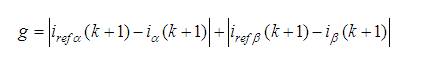
A two-level three-phase voltage source inverter is the least complicated multilevel inverter. The predictive current control of this type of inverter is done in order to provide an optimized system that controls the load current. In this case, the cost function is defined as,
The experimental results have been taken from [47], are shown in Figure 12.
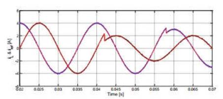
Figure 12. Experimental Result: Current Control of Inverter Using FS-MPC
Also current control method is applied to multilevel cascaded H-Bridge inverters [49]. Similarly, MPC is applied to PWM rectifier on unbalanced conditions in order to improve the DC side voltage and AC side current [50].
In[51, 52], the control of flying capacitor converter is presented using FS-MPC is presented. The control of matrix converter with 27 possible switching instants are proposed in [11].
Besides current control, power control is another approach for the control of power converters. As described in [53, 54], the cost function evaluates the error between the active and reactive power, ie,
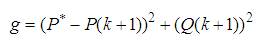
where the active power reference value is obtained from DC link voltage and reactive power reference is assumed to be zero. Based on the above cost function, the controlling process is done using MPC.
A review of predictive control schemes have been presented in this paper. These schemes are broadly classified into four categories i.e. hysteresis, trajectory, deadbeat, and model based predictive control (continuous and finite set MPC). The functional principles of all types of schemes have been described along with some examples. The hysteresis and trajectory based scheme are closely related to each other. Predictive control in comparison to other conventional controllers is considered as best for the control of power converters due to its various advantages i.e. easy inclusion of nonlinearities, constraints as well as no requirement of cascaded structure. It provides a fast dynamic response. According to the application and system requirement, the type of predictive control scheme is used. Thus, it can be concluded that, predictive control strategy will play a significant role in the development of converter and drive systems.