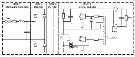
Figure 1. Typical CFL Ballast Circuit
Compact fluorescent lamps (CFLs) are increasingly being used in households and commercial buildings because of the desire to reduce electricity usage. CFLs are nonlinear, which raises concerns over the widespread use of CFLs due to possible adverse effects on harmonic voltage levels in the distribution system. A MAT LAB model of a simple CFL ballast circuit is shown to match actual CFL current waveforms and is used to assess the interactions between multiple CFLs connected to an electrical network. This work shows the error of using fixed harmonic current injection to model CFLs in a distribution system. Finally, the concept of CFL tensor analysis with phase dependency is introduced.
The desire to reduce electrical loading by using energy efficient lighting has resulted in a high level of interest in replacing conventional incandescent lamps with compact fluorescent lamps (CFLs). The use of CFLs is expected to save up to 10% of a household's electricity usage. Due to the non-linear characteristics of the electronic ballast, the CFLs will inject harmonic currents into the distribution system. The overall effect of these harmonic current injections at the distribution level could result in unacceptable voltage distortion at some points in the network. The combined effects of all these small sources can be just as detrimental as one large source, and is even harder to mitigate due to their distribution nature.
A few contributions have focused on the harmonic characteristics of CFLs, which are different from case to case because of the variety of ballast circuitry [1-5]. A number of other studies on CFLs have concentrated on the internal electronic ballast design to enhance their performance[6-8]. Some researchers have performed field experiments as well as direct harmonic simulation to investigate the possible effects of CFL harmonics on the local feeder or distribution network[9-10]. This paper categorizes CFLs based on the ballast circuit design to analysis their electrical characteristics. This is followed by modelling the CFL in MAT LAB to show the effect of interaction between multiple CFLs. The detailed simulations illustrate the error of using fixed harmonic current injection to model the CFL [11]. Finally, the phase dependent behaviour of CFL is discussed using tensor analysis.
There are two basic types of ballasts: low-frequency magnetic ballasts and high-frequency electronic ballasts. The functions of the two types of ballasts are essentially the same; that is, they control the starting and operating characteristics of the electricity for the appropriate fluorescent lamp. The primary difference is in the frequency delivered to the lamps and, obviously, the components that generate the frequencies.
The magnetic ballast uses a magnetic transformer of copper windings around a steel core to convert the input line voltage and current to the voltage and current required to start and operate the fluorescent lamps. Capacitors are added to assist lamp starting and power factor correction. But the output frequency is the same as the input frequency (50Hz).
An electronic ballast use integrated circuitry to perform all functions of the ballast. It rectifies the 60 Hz AC input to DC and then produces a very high-frequency current (20,000 -50,000 Hz) using an inverter and power conditioning components. In most models, the electronics is also used to provide the current limitations, and improve power factor. Use of controllable integrated circuits in an electronic ballast allows the output to be varied and the fluorescent lamps dimmable in response to manual or automatic (sensor) control. Some “hybrid” ballasts use some electronic circuitry to produce the high frequency current but use conventional current limiting and power factor correction components.
Complex electrical loads (other than simple resistive loads) have elements that change the ratio of the useable power to the supplied power. In other words, more supply power is required than is utilised. This is defined as the power factor. Most utilities penalise companies that have a low power factor. Both magnetic and electronic ballasts have components that reduce the power factor ratio2; in some cases, it is less than 85%. Electronic ballasts are now capable of power factor ratings of over 95% (some manufacturers claim greater than 99%). When purchasing ballasts it is important to ensure they have a power factor equal to or greater than 95% [12].
Many electrical devices, especially electronic devices, can produce a harmonic distortion of the shape (sine wave) of the electric wave form. This distortion degrades the quality of the electricity and can subsequently decrease the effectiveness and efficiency of the equipment. Total Harmonic Distortion is defined as a ratio of the sum of all the harmonics over the magnitude of the fundamental power. Most magnetic ballasts have a total harmonic distortion between 18% and 35%. Most electronic ballasts have the total harmonic distortion below 20% with some below 10%. It is advised to purchase ballasts that have low distortion specifications [13].
Figure 1 displays a block diagram of typical CFL ballast available in India. The first block contains the protection, filtering and current peak limiting components. Block 2 is the full diode bridge filter to the converter the ac line into a dc stage. Block 3 is the smoothing capacitor with a typical value of either 4.7 μF or 10 μF. It provides the DC input voltage of the resonant inverter for the tube in block 4. The diac is for starting the resonant inverter and the PTC (Positive Temperature Coefficient thermistor) for prolonging tube life. The PTC has a low impedance when cold ensuring the voltage is low across the tube and does not try to strike, causing a large current to flow through the electrode, thereby heating them up. When sufficiently heated the PTC becomes a high impedance allowing the tube to strike (typically after a second). The resonant inverter normally runs at 10-40 kHz, and this appears as a constant load as far as the DC busbar is concerned. This means that to investigate the harmonic currents on the AC input, only the first three blocks need to be represented in detail, and the resonant inverter and tube can be represented by a resistor [13].
There is a compromise between the generation of harmonics and cost, and often CFL life-time. The ripple on the DC voltage, measured by the crest factor (peak divided by RMS value), influences tube life. Increasing the filter capacitor reduces the ripple but increases the peakiness of the AC current waveform and hence the harmonics in it. Some other ballast designs also reduce the harmonic content but increase the crest factor. Addition of filtering or using a more sophisticated design can reduce the harmonic content but also increases the complexity and cost of the CFL. CFLs can be divided into four main categories in terms of their ballast circuitry and their attempt on improving the power-factor [14].
Figure 1. Typical CFL Ballast Circuit
Figure 2 shows a simple CFL with no filtering and hence nothing to improve the power-factor. Sometimes even the resistor in the ac lead is the absence, and the source impedance is relied upon to limit the capacitor charging peak. This circuit has very high harmonic current levels, which depend on the dc capacitor size and R, but is the cheapest to manufacture.
One way of increasing the ballast power-factor and to reduce the harmonic content of the input current waveform is the use of passive filtering. There are many types of passive filter arrangements, one of which is shown in Figure 3. Obviously, the more extensive the filtering is, the better the ac current waveform, but higher the cost. The advantage of this passive LC filtering technique is its simplicity and ease of implementation. However, the major drawback is the physical size and weight, which makes it unattractive due to the limited space and inherent power loss [15].
Another possible solution is to use valley-fill circuit (or equivalent), shown in Figure 4. In this circuit, the filter capacitor following the diode rectifier is split into two different capacitors C1 and C2, which are alternately charged and discharged using the three diodes. However, this circuit contains large DC voltage ripple, which produces lamp power and luminous flux fluctuation. As a result, it will reduce the lamp's lifetime.
The improved valley-fill circuit shown in Figure 5 adds to two identical small capacitors C3 and C4 as a voltage doubler to enhance the current waveform near crossover point. It continues to draw the current from the ac source during the cross-over period, which helps to extend the input current conducting angles. One resistor is connected to the bottom of C2 in order to remove the charging current spikes at the voltage peak. This is a cost effective way of improving power factor as well as reducing the harmonic current injection level [16].
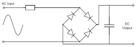
Figure 2. Simple CFL Ballast Circuit with no Filtering
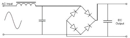
Figure 3. Passive Filtering Circuit
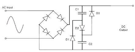
Figure 4. Valley-Fill Filtering Circuit
The measured harmonic spectra of more than 100 CFLs has allowed the identification of four categories of CFL; poor, average, good and excellent, which are associated with the ballast circuits used (Section II). Typical timedomain waveforms and their corresponding harmonic spectra as recorded and displayed in Figure 6.
Although CFL can be made virtually distortion free, the cost of doing it is significant. An ongoing debate between equipment manufacturers and electricity companies, and also in standards setting bodies, is where to draw the line regarding acceptable power quality and cost [17].
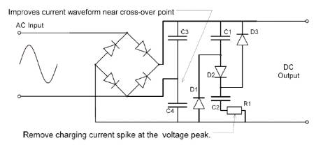
Figure 5. Improved Valley-Fill Circuit
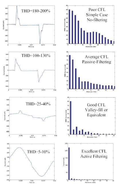
Figure 6. Typical Waveforms and Spectra for different classes of CFL Circuits
Figure 7 displays a comparison between a detailed MATLAB model of a simple CFL without power factor correction (Figure 2) with a resistive load and two brands of CFLs tested. Having verified the accuracy of the MATLAB model with lab measurements, this simple CFL model will be used to assess the interaction of multiple CFLs.
Harmonic analysis in time-domain involves simulation to steady-state, then using FFT to extract the harmonic components. The simplest way of modelling the CFL in a distribution system is to use fixed harmonic injection method, where the CFL is modelled by an ideal current source. Such representation is assessed by connecting a detailed CFL model to a stiff system network with zero impedance, then using the resulting harmonic current as the CFL fixed harmonic injection level along the distribution network shown in Figure 9. It assumes the harmonic voltage in the network has no effect on the CFL harmonic current. Hence, harmonic current injection at load 1 and 2 are identical to load point 0.
In order to consider the interaction between CFLs through the ac system, detailed simulation using the verified simple CFL model at each load point is used, as depicted in Figure 9. The harmonic injections from CFL 1 and CFL 2 are I_CFL_1 and I_CFL_2, respectively.
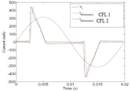
Figure 7. Verification of detailed MAT LAB model of a Simple CFL
The ac input current waveform of each CFL and their harmonic frequency components for the test system (Fig. 9) are depicted in Figures. 10 and 11 respectively, for a relatively strong system (R = 0.0075 Ohms, L = 8.0214e-5 H, Loading = 0.15 + j0.0075 p.u., Sbase=6.667 kVA, Vbase=400 V). It is important to note that the current waveform of the CFL at load point 0 is identical to the waveform of the CFLs for fixed injection (Figure 8), as the voltage is sinusoidal at this point. It is clear that a high frequency ringing appears on the waveform at approximately the 80th harmonic. Near this resonance, there is a large discrepancy between the fixed harmonic current injection and the detailed model. In practice, this would not be a problem as the natural low pass nature of the transformers (due to the neglected inter-turn capacitance) would damp this.
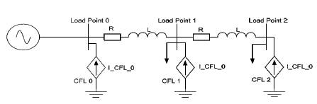
Figure 8. Fixed Harmonic Current Injection Representation.
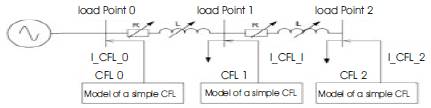
Figure 9. Test System 1 for showing CFLs Interaction
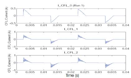
Figure 10. Current waveform of CFLs from Detailed Simulation (strong system)
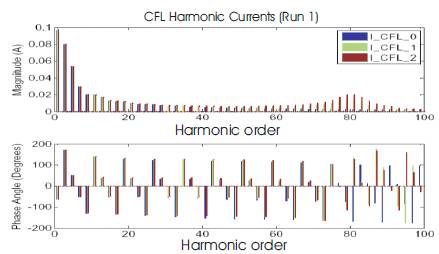
Figure 11. Current Spectra of CFLS from Detailed Simulation (strong system)
Figures 12 and 13 depict the same simulation with a weaker ac system (by a factor of 10 times). The resonant frequency, occurred between the inductive ac system and dc filtering capacitor in the CFL circuitry, is now around 27th harmonic and this will propagate through the network more easily and is of greater concern. This resonance is also obvious if the harmonic voltage spectra is inspected. Although the dc filter capacitor is connected via a diode bridge to the ac system, it still appears as a capacitance, the effective value being a function of the conduction period of the diodes. One common feature is that the phase angles of the injected harmonic currents from the CFLs are all in-phase below this resonance point yet seems out of phase above the resonance point. The double peak waveform seen in Figure 13 has been observed in measurements taken from the standard power outlet (domestic supply). These measurements are shown in Figure 14.
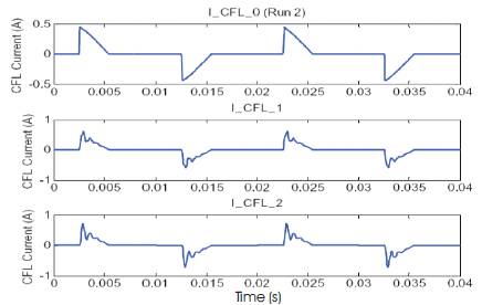
Figure 12. Current waveform of CFLs from Detailed Simulation (weaker system
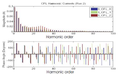
Figure 13. Current Spectra of CFLs from Detailed Simulation (weaker system)
For this test system, the ac system impedance is identical and the harmonic currents at load point 2 are compared to three times the harmonic currents produced by one CFL (load point 1). From this comparison it is clear that harmonic currents at load point 2 are not equal to three times of harmonic currents at load point 1. Hence in the 3 CFL case, the harmonic currents injected by one CFL has been influenced by the presence of the other two CFLs fed from a common ac source. The previous examples have illustrated that the CFLs harmonic injection depends on the network configuration as well as other nonlinear sources. Fixed harmonic current injection method will often overestimate or underestimate the harmonic injection level. These interactions can be described in the harmonic domain with the use of tensor representation to describe the phase dependency.
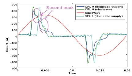
Figure 14. Measurements with Typical Domestic Supply
This paper has looked at the power-factor and harmonic performance of CFLs and linked this to the typical ballast topology. It has demonstrated the phase-dependent nature of CFLs whereby they are influenced by supply voltage distortion. This means there will be interaction between multiple CFLs through the ac system impedance and hence the direct harmonic current injection method will be inaccurate. A better approach for analyzing CFL, using tensor analysis, has been introduced. Tensor analysis opens the door to more accurate analysis of the impact of widespread CFLs use in distribution systems.