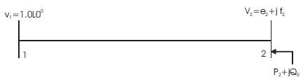
Figure 1. The Two Bus System
In this paper, attempts have been made to analyze and understand the voltage stability problem in a radial distribution system. Till now only constant power load model has been used to analyze the voltage stability problem of distribution system. However, in a distribution system the power demand for almost all the loads, which are connected, such as television, refrigerators etc. are voltage dependent in nature. Hence, for analyzing the voltage stability problem in a radial distribution system, it is more proper to take into account the voltage dependent characteristics of the loads instead of the constant power characteristics of the loads.
Distribution systems are the networks that transport the electric energy from bulk substations (or) sources to many services (or) loads. 30% to 40% of total investments in the electrical sector go to distribution system. The modern power distribution system is constantly being faced with an ever-growing load demand. Distribution systems experience distinct change from a low to high load level everyday. A major concern in power networks, which has surfaced fairly, recently is the problem of voltage stability. Due to the rapid growth in power demand of certain industrial power networks, incidence of unexpected voltage collapse is experienced. When such incidence happens, some industrial loads will be disconnected through automatic cut-off switches resulting in severe interruptions.
When the load demand (active or re-active) in a system increases, the voltages in the different buses in the system decrease. If the load demand in the system increases progressively, the bus voltages also decrease progressively, until a sharp accelerated decrease in the magnitude of the bus voltages take place. When this happens, the overall voltage in the system becomes very low and hence, the voltage in the system is said to have “collapsed” or voltage in the system is said to be “unstable”. Clearly, this low voltage in the system is an infeasible operating point.
Literature survey shows that a lot of work has been done on the voltage stability analysis of transmission systems [1], but hardly any work has been done on the voltage stability analysis of radial distribution networks. Jasmon and Lee [2] and Gubena and Strmcnik[3] have represented the whole network by a single line equivalent. The single line equivalent derived by these authors [2,3] is valid only at the operating point at which it is derived. It can be used for small load changes around this point. However, since the power flow equations are highly nonlinear, even in a simple radial system, the single line equivalent system representation would be inadequate for assessing voltage stability limit. In addition, their techniques [2,3] do not allow for changing loading pattern of the various nodes, which would greatly affect the collapse point
Reference [4] has shown the difference between system instability and radial voltage instability and that both problems can be solved by appropriate load shedding. Sterling et al. [5] have studied the voltage collapse at a load bus using the Thevenin equivalent circuit with respect to load bus concerned. In [5], by applying maximum power transfer theorem, a voltage collapse proximity indicator is derived.
In a distribution system, the real and reactive power consumed by the connected loads such as television, refrigerator, air-conditioners, heaters, fluorescent tube light, pump, motors etc. have a voltage dependent characteristic, i.e. as the voltage across these loads varies, power consumption by the loads also varies.
In this paper, an attempt has been made to determine the effect of the voltage dependent characteristics of the connected load on the voltage stability margin of a radial power distribution system. For constant power loads, a simple algebraic criterion for determining whether a distribution system is voltage stable or not at its present operating condition is derived. Based on the criterion, a simple computer algorithm to determine the voltage stability limit of a radial power distribution system is described. Suitable modifications of this algorithm for considering the voltage dependent characteristic of the loads is also proposed in this paper. A comparative analysis of the results regarding the voltage stability limits for constant power loads and voltage dependent loads is given in this paper.
The ability to predict the voltage collapse is most important, as it can save the system from an unwarranted eventuality. The voltage instability problem is due to the voltage drop that occurs when the loading on a radial network exceeds its capacity for controlling the receiving end voltage. It is possible to reduce a distribution system to an equivalent two-bus system and subsequently predict the voltage stability limit of the original system from the voltage stability property of the equivalent two-bus system. In the subsequent sections, the algorithms for derivig an equivalent two-bus system from a radial distribution system for constant power loads and voltage dependent loads are described.
Let us consider a two-bus system as shown in Figure1. Bus 1 is the substation bus and the voltage of bus 2 is expressed as e2 + jf2 The power demand at bus 2 is P2 + jQ2.
Figure 1. The Two Bus System
The power flow equations in the rectangular form are expressed as

Where yij =Gij – jBij and

From eqns (1) and (2) and noting that e1 +jf1 = 1.0+j0, we Have
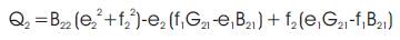
Using eqn (3), eqns (4) and (5) can be re-written as,
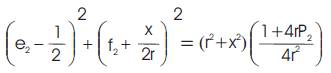
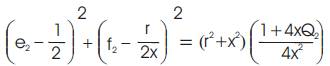
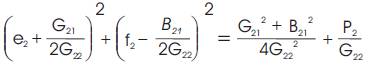
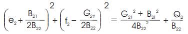
Eqns (6) and (7) define two circles on the e2 -f2 plane, with
centers at (1/2, -x/2r) and (1/2, r/2x) respectively and radii
of 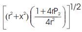 and
and 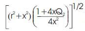 respectively
The intersection points of these two circles represent the solution points of e2 & f2 . If the solutions for e2 and f2 exist, then these two circles must intersect each other. Thus, the condition for existence of the solution is,

Simplifying eqn (8) we get,
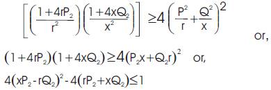
Eqn (9) is the condition for voltage stability in the two-bus system.
To use the condition for voltage stability of a two-bus system for predicting the voltage stability, it is necessary to find an equivalent two-bus system of a given radial distribution network. The technique by Baran and Wu [6] is used to derive such an equivalent network as follows.
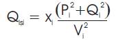
1.2.1 Main FeederConsider that a distribution system consists of only a radial main feeder as shown in Figure 2.
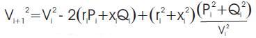
The voltage profile, real and reactive power losses are calculated using eqns.(12), (13) and (14) respectively. These equations are iteratively computed. These equations are called load flow equations.
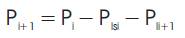
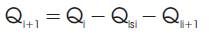
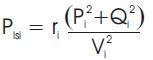
Where Pl sl and Ql sl are real and reactive power losses in the branch emanating from bus i and Pli and Qli are the real and reactive power demand.
1.2.1.1 Algorithm for Equivalent Two-Bus SystemUsing eqns (10)-(14), an equivalent two-bus network can be derived from Figure 2 as shown in Figure 3. The algorithm described as follows can compute the equivalent resistance and reactance:
Step 1: Sum the entire load demands on each bus in Figure 2. Let this term be the initial power injection (P1 +jQ1 ) for the substation bus in Figure 2 as well as the load demand (P2' +jQ2' ) in Figure 3.
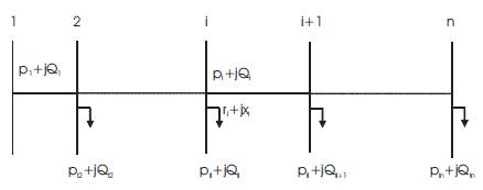
Figure 2. A Radial Distribution System Comprising of one Main Feeder
Figure 3. The Two Bus Equivalent Network
Step 2: Starting from the substation bus, calculate the successive Pi+1 , Qi+1 , Vi+1 and the power losses Plsl , Qlsl in Figure 2 using eqns (10)- (14)
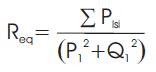
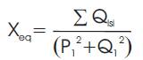
Step 3: Sum all these power losses and compute the equivalent impedance (Req +jXeq )
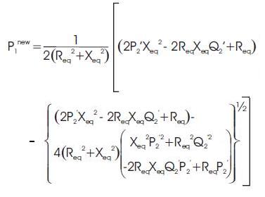
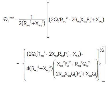
Step 4: Calculate the new power injection of the equivalent 2- bus network by using equations,
Step 5: Compare P1new & P1 which was obtained from step 1, if (P1new - P1 ) < tolerance, then stop. Otherwise, set P1 to P1new and Q1 to Q1new and return to step2.
1.2.1.2. Lateral feederConsider a main feeder with a lateral as shown in Figure 4. The same process for finding the equivalent network applied to the main feeder can be applied to the lateral branching out of node k also.
Step 1: Sum the entire load demands on each bus in Figure 4. Let this term be the initial power injection (P1 + jQ1 ) for the swing bus in Figure 4 as well as the load demand (P2' + jQ2' ) in Figure 3.
Step 2: Starting from the substation bus, calculate the successive Vi+1 and check whether any lateral exists at each bus i. If there is a lateral at that bus then go to step 3, otherwise go to step 4.
Step 3: Let there be a lateral at bus k. Sum all the real and reactive loads on the lateral at bus k. Let this term be denoted as Pko +j Qko . With the knowledge of the voltage on bus k, which has already been calculated from step 2, it is possible to calculate power flows, losses and the bus voltages on the subsequent sections and buses on that lateral. Sum up the losses on all the sections on that lateral. Add this loss term to Pko + jQko . Let the constant power load and the value of the load be Pkr + jQkr .
Step 4: Calculate the successive Pi+1 , Qi+1 and Vi+1 and the power losses, Plsl , Qlsl on the main feeder in Figure 4 from eqns (10) – (14).
Step 5: Sum all these power losses and compute the equivalent impedance (Req + jXeq ) using eqns. (15) and (16).
Step 6: By using eqns (17) and (18), calculate the new power injection of the equivalent two-bus network.
Step 7: Compare P1new & P1 , which was obtained from Step 1. If (P1new -P1 )< tolerance, then stop. Otherwise, set P1 to P1new and Q1 to Q1new and return to step 2.
From the discussion of section 1.2, it is obvious that the algorithm described is suitable only for constant power loads. However, as discussed earlier in a practical distribution system the connected loads are often not of constant power type. Rather, they are essentially voltage dependent loads and expressed by the following equations

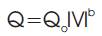
Where P & Q are real and reactive parts of the loads at a voltage magnitude V. P0 and Q0 are the loads at the initial operating condition. 'a' & 'b' are the suitable exponents. The typical values of 'a' & 'b' for different loads are shown in Table .1 [6]
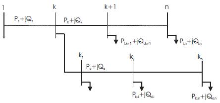
Figure 4. A Radial Distribution System with laterals
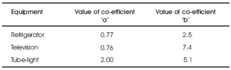
Table 1. Coefficients of 'a', 'b'.
When the distribution system comprises only one main feeder with voltage dependent loads it is as follows.
Step 1: Assume flat voltage profile in the system initially. As the exponents 'a' and 'b' and the values of P0 and Q0 are specified at each load bus, the effective real and reactive load demand at each bus can be calculated. Sum the load demands on each bus. Let this term be the initial power injection (P1 + jQ1 ) for the sub-station bus in Figure 2 as well as the load demand (P2' + jQ2' ) in Figure 3.
Step 2: Starting from the substation bus, calculate the voltage at the next bus by using eqn (12). After the voltage is calculated, the effective real and reactive power at that bus is calculated using eqns (19) and (20). Once these load demands are calculated, the power flows and the losses over the next feeder section can be calculated.
Step 3: Repeat step2 for all the subsequent buses and the feeder section. Once the new load demands at all the buses are calculated, add these new load demands and set the result equal to load demand (P2' + jQ2' ) in Figure 3.
Step 4: Sum all the losses and calculate the equivalent impedance (Req + jXeq )
Step 5: Calculate new power injections P1new & Q1new
Step 6: Compare P1new & P1 , which was obtained, form Step
1. If (P1new –P1 )< tolerance, then stop. Otherwise, set P1 to P1new and Q1 to Q1new and return to step2.
The algorithm is described as follows:
Step 1: Assume flat voltage profile in the system initially. As the exponents 'a' and 'b' and the values of P and Q are specified at each load bus, the effective real and reactive load demand at each bus can be calculated. Sum the load demands on each bus. Let this term be the initial power injection (P1 + jQ1 ) for the substation bus in Figure 4 as well as the load demand (P2 ' + jQ2 ') in Figure 3.
Step 2: Starting from the substation bus, calculate the voltage at the next bus by using eqn (12). Check whether any lateral exists at that bus. If there is a lateral at that bus then go to step 3, otherwise go to step 4.
Step 3: Let there be a lateral at bus k. Sum all the real and reactive loads on the lateral at bus k. Let this term be denoted as Pko + jQko . With the knowledge of the voltage on bus k, which has already been calculated from step 2, it is possible to calculate bus voltage, effective load at a bus. Sum up the losses on all the sections on that lateral, add this loss term to Pko + jQko . Let the resultant term be denoted as Pkr + jQkr . The original lateral would be replaced by a constant power load and the value of the load is Pkr + jQkr . The original lateral, having voltage dependent loads on it, is replaced by a constant load, as there is no easy method to compute aggregate or equivalent 'a' and 'b' coefficients for that lateral.
Step 4: Calculate the successive bus voltage, effective load at a bus, feeder section power flow and feeder section loss in that order for the subsequent buses and feeder sections on the main feeder in Figure 4 Once the new load demands at all the buses are calculated, add these new load demands and set the result equal to load demand (P2 ' + jQ2 ') in Figure 3.
Step 5: Sum all these power losses and compute the equivalent impedance (Req +jXeq ).
Step 6: Calculate the new power injection of the equivalent two-bus network.
Step 7: Compare P1new & P1 , which was obtained from step
1. If (P1new – P1 ) < tolerance, then stop. Otherwise, set P1 to P1new and Q1 to Q1new and return to step 2.
It is obvious that the stability limit of a system is always expressed in terms of the maximum loadability of the system. Consequently, if the real or reactive power loading at any bus of a distribution system is increased progressively, after a certain limit, the voltages at all the buses of the system would collapse. This maximum value of the load would be known as the stability limit of the system at that particular bus or the “bus stability limit”. Similarly it is possible to determine the “bus stability limits” at all the buses of the system. The step-by-step algorithm for determining the “bus stability limits” is given below.
Step 1: For the base loading condition, determine the equivalent two-bus network following the algorithm described in subsection 1.3.1.
Step 2: Check whether the system is voltage stable or not using eqn (9). If the system is voltage stable, go to step 3.Otherwise go to step 9.
Step 3: Choose any bus i of the system.
Step 4: Set Pi = PBi where Pi is the present real power loading at bus 'i' and PBi is the base real power loading at that bus. Increase the real power loading at bus 'i' by an amount P(0.01p.u). Keep the loading at all other buses constant at the level of the base loading condition. Hence Pi =PBi +P.
Step 5: After the two- bus equivalent system is obtained, check for voltage stability using eqn (9). If the system is stable, go to step 6. Else go to step 7.
Step 6: Set Pi =Pi +P and go back to step 5.
Step 7: The “bus stability limit” at bus 'i' is given by Pi . Set Pi =PBi
Step 8: Repeat steps 3,4,5,6 and 7 for the remaining buses of the system.
Step 9: Stop.
The step-by-step algorithm for determining the “bus stability limits” with voltage dependent loads is given below.
Step 1: For the base loading condition described above, determine the equivalent two-bus network following the algorithm described in section 1.3.2
Step 2: Check whether the system is voltage stable or not using eqn (9). If the system is voltage stable, go to step3. Otherwise go to step9.
Step 3: Choose any bus 'i' of the system.
Step 4: Set Pi0 = PBio , where Pio is the present initial real power loading at bus 'i' and PBio is the base initial loading at that bus given in Table B.1. Increase the initial real power loading at bus 'i' by an amount P. Keep the initial loadings at all the other buses constant at the level of the bus initial loading condition. Hence Pio = PBio +P
Step 5: Determine the two-bus equivalent of the system at this new loading condition. After the two- bus equivalent system is obtained, check for voltage stability using eqn (9). If the system is stable, go to step6. Else, go to step7.
Step 6: Set Pio = Pio +P and go back to step 5
Step 7: The “bus stability limit” at bus 'i' is given by Pio . Set Pio = Pbio
Step 8: Repeat steps 3,4,5,6 and 7 for the remaining buses of the system.
Step 9: Stop
To investigate the effects of the voltage dependent loads on the voltage stability of a radial distribution system, detail studies have been carried out on two different test systems.
The first test system, which has been undertaken for study is a 10-bus system [8]. The load data and the feeder data of this system are given in [8].
The bus stability limits for 10- bus system with constant power load is given in Table 2.
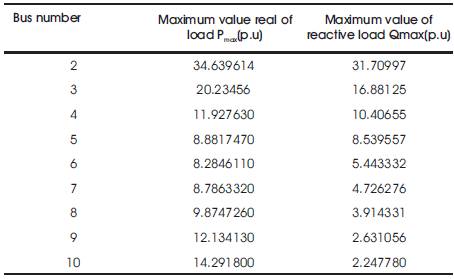
Table 2. Bus Stability Limits for 10-Bus System with Constant Power Loads
The “bus stability limits” (both real and reactive) are plotted with respect to the “electrical distance” of the buses from the substation as shown in Figures 6 and 7. The “electrical distance” of any bus from the substation is simply the modulus of the sum total of the impedances of the intermediate feeder sections, which need to be traversed to reach that particular bus from the substation.
It is observed from Figures 7 and 8 that the reactive power “bus stability limits” progressively decreases as the “electrical distance” increase. Hence, the farther a load point from the substation is, lesser would be its reactive power stability limit. On the other hand, the real power limits decrease up to a certain distance and beyond that these limits again increase. Also, from Table 2 it can be easily seen that the reactive power limits are always less than the real power limits. This seems to be appropriate as it is known that the voltages in any system is more sensitive to the reactive power demand in that system and voltage stability phenomenon is essentially a manifestation of the reactive power deficiencies in the system.
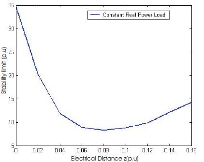
Figure 5. Real power bus stability limits for 10-bus system
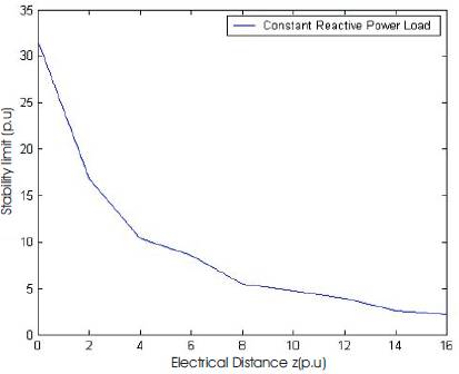
Figure 6. Reactive power bus stability limits for 10-bus system
The solution for the voltage of bus 2 has been obtained for different values of 'a' and 'b'. The results are tabulated in Table 3.
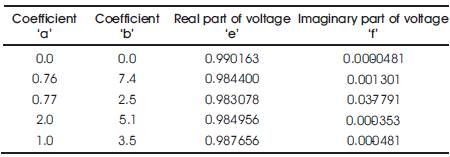
Table 3. Voltages at Bus 2 for different values of 'a' and 'b'
From Table 3 it is observed that the voltage of bus 2 does not change appreciably when different types of loads are connected at that bus. Hence, for the two-bus system, the stability condition given in eqn (9) can be used as an approximate condition for voltage dependent loads.
To find out the bus stability limit with voltage dependent loads for the 10 bus system voltage dependent loads are assumed arbitrarily as given in Table 4.
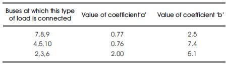
Table 4. 'a' and 'b' Coefficients at Different Buses
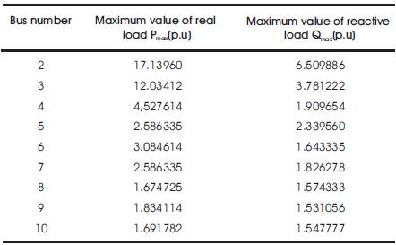
Table 5. Stability Limits with Voltage Dependent Loads in 10-Bus System
The results regarding the “bus stability limits” for various voltage dependent loads in the 10-bus system are tabulated in Table 5. Comparison of Tables 5 and 2 reveals that the stability limits of the system are lower for voltage dependent loads than the stability limits for constant loads.
The second test system, which has been considered for study, is a 31-bus system taken from [9]. The load data and feeder data of this system are given in [9]. The bus stability limits for this system with constant power load is given in Table 6. The variation of stability limit with electrical distance is shown in Figures 7& 8.
From Figures 7 & 8 it is observed that with the increase in the electrical distance, both the real and reactive power stability limits generally decrease. However, the limits do not vary in a smooth fashion as in the case of the first system with only one main feeder. Moreover, the reactive power stability limits also do not decrease monotonically as in the case of first system.
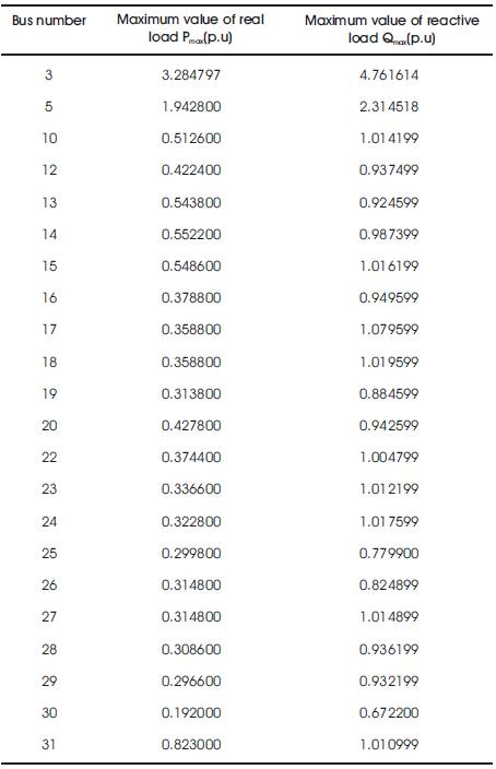
Table 6. Bus Stability limits for 31-Bus System with Constant Power Load
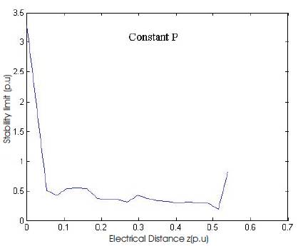
Figure 7. Real Power Stability Limit for 31-Bus System
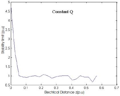
Figure 8. Reactive Power Stability Limits of 31-Bus System
The stability limits correspond to voltage dependent loads have also been found out for one set of 'a' and 'b' coefficients. These set of coefficients are tabulated in Table 7. The stability limits for this case is tabulated in Table 8.
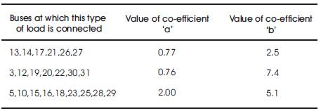
Table 7. 'a' and 'b' Coefficients at Different Buses
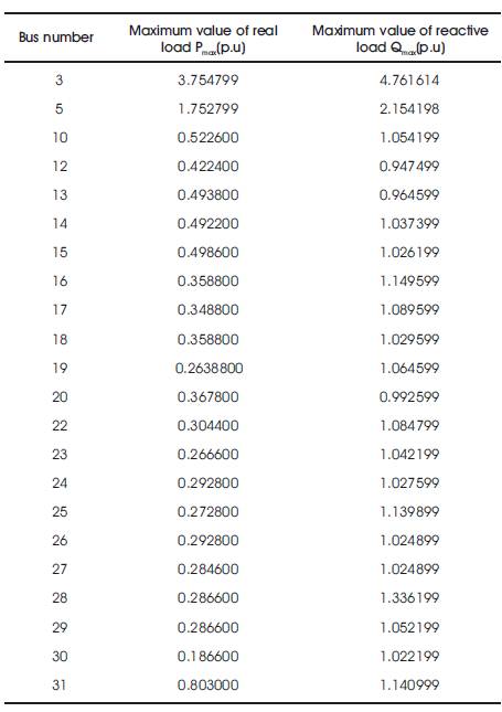
Table 8. Stability Limits with Voltage Dependent Loads in 31-Bus System
From comparison of Tables 2 & 8, it is found that at some buses the real power stability limits have decreased for voltage dependent loads, whereas on the other buses, these limits have increased. On the other hand, the reactive power stability limits have increased for voltage dependent loads as compared to the limits for constant power loads.
In this paper, a detailed investigation about the voltage stability limits in two different radial power distribution systems has been made. Two different types of loads, e.g. constant power loads and voltage dependent loads have been considered in both the systems. With the increase of distance of a load from the substation bus, the stability (both real and reactive) limits at that bus generally decrease. For a radial distribution system with only a main feeder, the reduction in the stability limits with distance is monotonic in nature. For radial distribution system with laterals present in the system, the reduction in the stability limits with distance is not monotonic in nature. But generally, the limits decrease with the increase in distance. Also the variation in the stability limits with distance is heavily dependent upon the particular system topology.