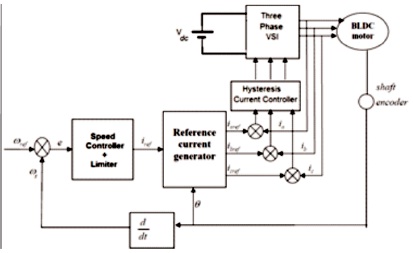
Figure 1. BLDC Motor Drive Control Scheme
This paper is aimed at the speed control of a Brushless Direct Current (BLDC) motor drive, for which a single loop control and cascade system of control is established and the performance of the drive system is compared. Initially, the drive system is modeled in a single loop using transfer function model. Then it is modeled with cascaded loops. Both the models are simulated using MATLAB/SIMULINK. Magnitude optimum multiple integration tuning method has been introduced for BLDC motor drive system to tune PID controller parameters. By performing various simulation tests with and without disturbances at supply side, load side and under set-point changes, the simulation results show that the cascade control system has better performance than single loop control no matter where the disturbances enter and sudden changes occur at the reference speed of the drive system.
BLDC motor has a wide range of applications because of its advantages, such as high efficiency, flat speed-torque characteristics, high speed range, smaller in size and lighter, longer life, low noise and good dynamic response when compared to brushed direct current motor. BLDC motor is a kind of permanent magnet synchronous motor (PMSM), trapezoidal type of PMSM is known as brushless direct current motor. In a brushless motor, stator contains windings and rotor incorporates permanent magnet. Moving the permanent magnets to rotor and driving field coils with power electronic switch can eliminate the brushes in DC motor (Merugumalla & Kumar, 2017). BLDC motors are often called as electronically commutated motors. It requires some electronic control mechanism to determine the rotor position continuously (Baszynski and Pirog, 2013). The rotor position can be determined either by measuring changes in back emf at each of the armature coils, which is known as sensorless control or by using a hall effect sensors embedded into the stator on the non-driving end of the motor (Stirban et al, 2012; Cui et al., 2014; Kim&Ehsani,2004; Merugumalla & Kumar,2018).
The control of motor drives was open-loop in 1950s, with the change in load effects the speed of the motor and sometimes the motor stall at low speeds. To overcome this difficulty, the closed-loop control of drives gain acceptance in industrial applications due to its accuracy and mastery of tuning the system to the desired performance. In the closed-loop control of the motor drive system, two loops exist namely inner-current loop and outer-speed loop. The PID controller has a highest priority in executing control of drives because its has simple structure and ease of operation (Taeib & Chaari, 2015; Astrom et al.,1992; Merugumalla & Navuri, 2016). The tuning of the controller must have the ability to deliver commands to the process for the perfect tracking of the reference with rejection of disturbances occur in the process during its operation. A good tuning method considers an adaptive behaviour of controller in case of uncertainties in the process and it is necessary for tuning procedure to achieve robust performance in terms of reference tracking and rejection of disturbances (Er et al, 2014). The tuning of PID controller parameters based on a known process model is an indirect tuning method, which extracts more information from the process for better tuning results (Nikranjbar, 2014). To the best information available from literature, MOMI tuning method for controlling the BLDC drive has not yet been implemented.
In this paper, the magnitude optimum multiple integration tuning method is proposed to tune the PID controller parameters. This method is an indirect method of tuning PID controller parameters. It extracts more information from process and provides non-oscillatory response. This method uses the concept 'Moments' (areas), which are calculated by the multiple integrations from open-loop response of the process (Vrančić et al, 1999b; Vrančić etal, 2001; Papadopoulos, 2015). These areas along with openloop process gain are used directly for the calculation of PID controller parameters. As the operation of BLDC motor involves nonlinear constraints and non-stationary conditions, this method adapts a solution for changing circumstances and gives robust response.
The schematic diagram of the basic BLDC motor driver control is shown in Figure 1. The motor drive system mainly consists of BLDC motor, three-phase voltage source inverter, hysteresis current controller, reference current generator and speed controller. The motor is supplied by the three phase voltage source inverter, and the switching functions obtained from the hysteresis current controller serve as input to the voltage source inverter. The reference currents i_aref, i_bref, i_cref are generated by reference current generator based on rotor position. The actual speed of the motor is compared with the reference speed and error is applied to controller and the controller output serves as the input to the reference current generator. The output voltages obtained from the three phase voltage source inverter, which can be expressed in the form of switching functions. BLDC motor, load and inverter are modeled and derived by combining the transfer function of BLDC drive system. (Kaliappan, 2015; Eti & Kumar, 2014; Ji & Li, 2009; Merugumalla & Navuri, 2019).
Figure 1. BLDC Motor Drive Control Scheme
The voltage per phase applied to BLDC motor is,
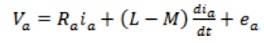
Where, L-self inductance, M-mutual inductance, Ra - resistance and ea -back emf
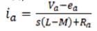
Applying the Laplace Transform to equation (1) and neglecting the initial conditions, the current per phase of motor will be given as,
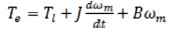
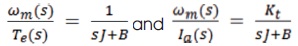
The electro magnetic torque equation is,
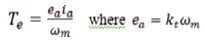
and
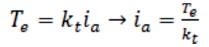
From the block diagram shown in Figure 2, transfer function of motor and load can be obtained as follows.
Figure 2. BLDC Motor and Load Model
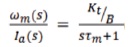
by taking Tm = J/B in equation (7), then
The transfer function of load can be obtained as,
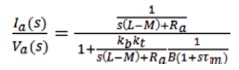
and to derive the transfer function of BLDC motor:
The transfer function of an inverter is,
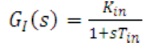
Where,
Vdc - DC link voltage input to inverter
Vcm - Maximum control voltage
fc – Switching or carrier frequency
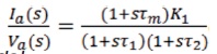
After approximation, the current loop transfer function  is obtained as follows.

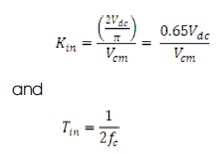
The transfer function of speed controller is given by,
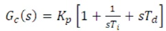
A Magnitude Optimum Multiple Integration (MOMI) tuning method is an indirect method of tuning PID controller parameters. This method is straight forward and simple and is based on the open-loop process output during step change in the process input. (Damir et al, 1999b). The tuning procedure for the PID controller is given for those processes which can be approximated by the following transfer function.
where, Kpr denotes the process steady-state gain, and a1 to an and b1 to bm are the corresponding parameters (m ≤ n) of the process transfer function, where 'n' denotes an arbitrary positive integer value. The direct identification of Kpr, a1 to an, b1 to bm is complex and difficult, to overcome such difficulty, MOMI method uses the concept 'moments (areas)', which can be expressed by integrating the process open-loop step response after applying the stepchange (dU) at the process input at t=0. (Vrančić et al., 2001; Vrančićet al., 2010). The graphical representation of moment (area) is shown in Figure 3 where y0 and u0 represents scaled process output and process input time, respectively.
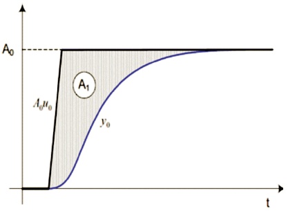
Figure 3. Graphical Representation of Moments (Areas)
The process transfer function can be expressed as areas by using the following infinite-order expression.
where, parameters A (i = 0, 1, 2, …) represent the time- i weighted integrals of the process impulse response. In practice, the process can be easily parameterised by the moments Ai (Vrančić et al., 1999a). The moments A1, A2, A3 A4, A5 can be calculated directly from the process transfer function after determination of process steady-state gain (Kpr) from process output.
The process steady-state gain is calculated from the process output as,

By using areas A1 to A5, the PID controller parameters can be calculated as,
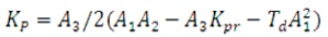
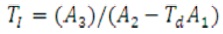
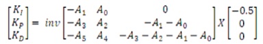
The PID controller tuning procedure is as follows.
By substituting the values of BLDC drive specifications from appendix in equations (8), (10) and (11), the transfer function of motor, inverter and load can be determined as, The transfer function of BLDC motor is,
The block diagram of single loop control is shown in Figure 4. The overall transfer function of BLDC motor drive system (process) using block reduction rules is determined as follows.
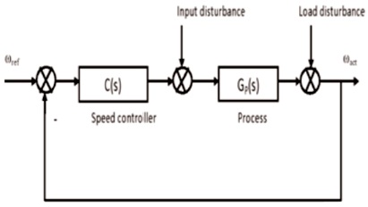
Figure 4. Block Diagram Single Loop Control
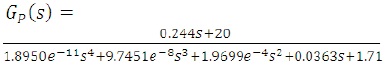
From the process transfer function, a0 =1.71, a1 =0.0363, a2 = 1.9699e-4, a3 = 9.7451e-8, a4 = 1.8950e-11, b0 = 20, b1 =0.244.
The open-loop process input is shown in Figure 5 and open loop process output response is shown in Figure 6, from which steady-state process gain KPR = A0 can be determined. With KPR, areas A1 – A5 and PID controller parameters which can be calculated from equations (17)-(21) and equation (25), respectively are presented in Table 1.
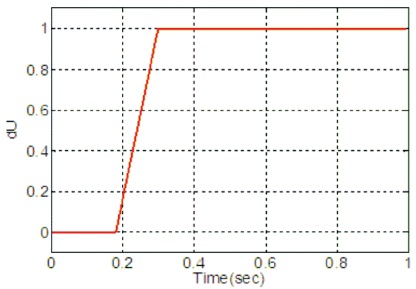
Figure 5. Open-loop Process Input Response
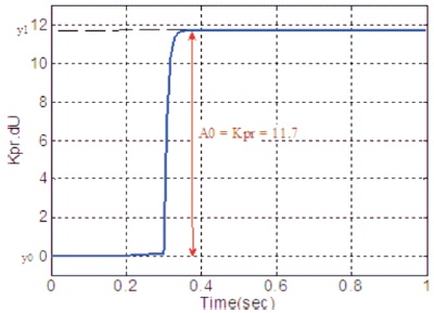
Figure 6. Open-loop Process Output Response
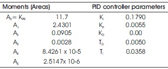
Table 1. Calculated Areas and PID Controller Parameters
The MATLAB/SIMULINK model of cascaded BLDC drive is shown in Figure 7. The overall BLDC drive process G(s) = G1(s) G2(s) is split into G1(s) and G2(s).
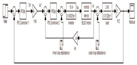
Figure 7. Simulink Model of Cascade Control System
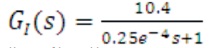
The inner loop process (inverter and BLDC motor) transfer function is,
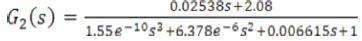
From transfer function a0 =1, a1 =0.006615, a2 =6.378*10-6, a3 =1.55*10-10, b0=2.08, b1 =0.02538.
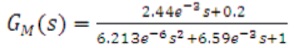
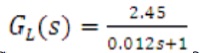
The outer loop process (load) transfer function is,
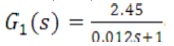
From transfer function a0 =1, a1 =0.012, b0 =2.45.
The open-loop process input and output of inner loop is shown in Figure 8, from which steady-state process gain Kpr = 2.08 is obtained. With known value of process gain, the areas A1 to A5 are calculated using equations (17)–(21). With these areas, PID controller parameters are calculated using equation (25).
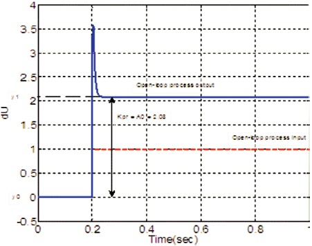
Figure 8. Open-loop Process Input and Output Responses of Inner-loop
The calculated areas and controller parameters for the inner loop are presented in Table 2.
Table 2. Calculated Areas and Controller Parameters of Inner-loop
The open-loop process input and output of outer loop is shown in Figure 9, from which steady-state process gain Kpr = 2.45 is obtained. With this value of process gain, the areas A1 to A5 are calculated using equations (17)–(21). With these areas, PID controller parameters are calculated using equation (25).
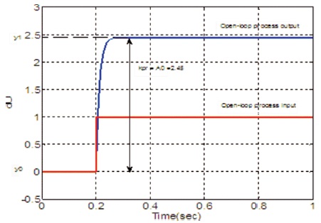
Figure 9. Open-loop Process Input and Output Responses of Outer Loop
The calculated areas and controller parameters for the outer loop are presented in Table 3.
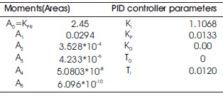
Table 3. Calculated Areas and Controller Parameters of Outer Loop
First, single-loop control and cascade control without any disturbance is implemented to control the BLDC motor. The reference speed is set to 73.33 rad/sec. The speed responses of a single loop and cascade control are shown in Figure 10. Cascade control shows better performance in terms of settling time and steady-state error compared to single-loop control.

Figure 10. Speed Response Without Disturbance
Second, single-loop control and cascade control with the disturbance considered on the supply side of the motor at 2s. The speed responses of single loop and cascade control with disturbance is shown in Figure 11, it can be seen that single-loop control contains overshoot where as cascade control does not shows any overshoot.
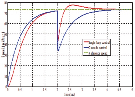
Figure 11. Speed Response With Disturbance at Supply Side
Third, single-loop control and cascade control with disturbance considered on load side of the motor at 2s. The speed responses of single loop and cascade control with disturbance is shown in Figure 12, with the same magnitude of disturbance, it can be seen that the effect of disturbance is less in cascade control compared to single-loop control.
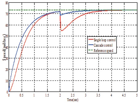
Figure 12. Speed Response With Disturbance at Load Side
Fourth, the reference speed is initially set to 30 rad/sec and suddenly at 2.5s, speed is increased to meet final speed of 73.33 rad/sec. The speed reference tracking is better with cascade control compared to single-loop control, which can be seen in Figure 13.
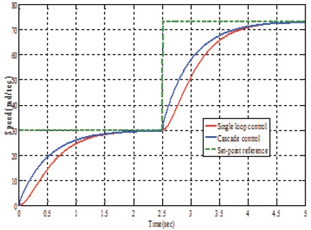
Figure 13. Speed Response With Set-point Change
In this paper, the single-loop control system of BLDC motor drive is compared to cascade control system. The motor drive system consisting of motor, inverter and load that can be modeled using transfer function model of each component and the overall drive system. Initially, drive system is modeled in a single loop using transfer function model. Later, the drive system is modeled with cascaded loops. Both the models are simulated using MATLAB/ SIMULINK. Several simulation tests like introducing disturbances at supply side, load side, and at set-point changes were investigated the performance and robustness of single loop and cascaded loop control systems. Cascade loop control system shows less effect of disturbances at supply side and at load side. The reference speed tracking under set-point changes is also tested and results demonstrate the prominence of cascade control system over single-loop control system of BLDC motor drive.