(1)
The problem of voltage deviation and power loss is mostly addressed in distribution system by growing domestic, industrial and commercial load day by day. To minimize these problems, effective planning of distribution system is required. This effective and reliable planning of distribution system is achieved by optimized placement of control device (capacitor) in distribution networks. The idea for optimal capacitor placement is determined with the location of the capacitor to be installed in the distribution network buses where power losses should be minimum and cost saving should be maximum. This paper presents a new and efficient approach for capacitor placement in radial distribution systems that determine the optimal locations and size of capacitor with an objective of improving the annual cost saving, the voltage profile and reduction of power loss. The solution methodology includes an algorithm that employs Plant Growth Simulation Algorithm (PGSA) and Genetic algorithm to estimate the optimal size of the capacitors at the optimal buses determined. The effectiveness of the proposed method is applied to 33 and 69 bus IEEE radial distribution systems. Result shows that after placement of capacitor in candidate buses the energy loss has been reduced.
Dr N.Visali et.al, in their work “Loss Reduction in Radial Distribution System by Optimal Placement of Capacitor using Differential Evolution Method,” proposed optimization method (differential evolution) for capacitor placement in radial distribution system [1]. A.Kartikeya Sarma and K.Mahammad Rafi in their work “Optimal Selection of Capacitors for Radial Distribution Systems using Plant Growth Simulation Algorithm,” explained the importance of capacitor sizing and selection for radial distribution system to reduce the losses and cost savings [2]. The loss minimization in distribution systems has assumed greater significance recently since the trend towards distribution automation will require the most efficient operating scenario for economic viability variations. Studies have indicated that as much as 13% of total power generated is wasted in the form of losses in the distribution level. To reduce these losses, shunt capacitor banks are installed on distribution primary feeders. The advantages with the addition of shunt capacitors banks are to improve the power factor and feeder voltage profile. Power loss reduction increases the available capacity of the feeders. Therefore it is important to find out the optimal location and sizes of capacitors in the system to achieve the above mentioned objectives. Mr. Manish Gupta and Dr. Balwinder Singh Surjan in their work “Optimal sizing and Placement of Capacitors for Loss Minimization In 33-Bus Radial Distribution System Using Genetic Algorithm in MATLAB Environment,” proposed the method of genetic algorithm for capacitor placement and sizing in radial distribution system [3]. Since, the optimal capacitor placement is a complicated combinatorial optimization problem, many different optimization techniques and algorithms have been proposed in the past. Schmill [4] in his work “Optimum Size and Location of Shunt Capacitors on Distribution Feeders,” developed a basic theory of optimal capacitor placement. The author presented his well-known 2/3 rule for the placement of one capacitor assuming a uniform load and a uniform distribution feeder. H. Dura [5] in his work “Optimum Number Size of Shunt Capacitors in Radial Distribution Feeders,” considered the capacitor sizes as discrete variables and employed the dynamic programming to solve the problem. J.J. Grainger and S.H.Lee [6] in their work “Optimum Size and Location of Shunt Capacitors for Reduction of Losses on Distribution Feeders” developed a nonlinear programming based method in which capacitor location and capacity were expressed as continuous variables. J.J. Grainger and S. Civanlar [7] in their work “Volt/var control on Distribution systems with lateral branches using shunt capacitors as Voltage regulators” formulated the capacitor placement and voltage regulators problem and proposed decoupled solution methodology for general distribution system. M.E.Baran and F.F.Wu [8] in their work “Optimal Sizing of Capacitors Placed on a Radial Distribution System,” presented a method with mixed integer programming. Sundharajan and Pahwa [9] in their work “Optimal selection of capacitors for radial distribution systems using genetic algorithm,” proposed the genetic algorithm approach to determine the optimal placement of capacitors based on the mechanism of natural selection. In most of the methods mentioned above, the capacitors are often assumed as continuous variables. In distribution system to improve the voltage regulation it is required to minimize reactive power flow through the system. To overcome these difficulties the capacitor placement is essential in distribution system. The placement of capacitors in radial distribution systems, also provide power flow control, improving system stability, power factor correction, voltage profile management and losses minimization. In this paper, Capacitor Placement and Sizing is done by Loss Sensitivity Factors and Plant Growth Simulation Algorithm (PGSA) respectively. The loss sensitivity factor is able to predict which bus will have the biggest loss reduction when a capacitor is placed. Therefore, these sensitive buses can serve as candidate locations for the capacitor placement. PGSA is used for estimation of required level of shunt capacitive compensation to improve the voltage profile of the system. The proposed method is tested on 33 and 69 bus radial distribution systems and results are very promising. The advantages with the Plant Growth Simulation Algorithm (PGSA) is that it treats the objective function and constraints separately, which averts the trouble to determine the barrier factors and makes the increase/decrease of constraints convenient, and that it does not need any external parameters such as crossover rate, mutation rate, etc. It adopts a guiding search direction that changes dynamically as the change of the objective function. The remaining part of the paper is organized as follows: Section 1 gives the objective function; Section 2 Load Flows; Sections 3 explains system description, Sections 4 Solution Methodology gives brief description of the plant growth simulation algorithm and Genetic algorithm; Section 5 develops the test results and Section 6 gives conclusions.
The aim of the present work is to find out annual cost savings & loss minimization using optimization techniques. Therefore the objective function consists of two terms: 1) capacitor cost and 2) loss minimization.
Capacitor cost is divided in to two terms: cost installation cost and variable cost which is proportional to the rating of capacitors. Capacitor cost ( c ) is
Where Ci is the installation cost of the capacitor
Cv is the rate of capacitor per KVar
Qk is the rating of capacitor in particular bus let kth bus
If I is the current in particular section let I in time duration T, then energy loss in section is
ELi is the energy loss in section i
Ii is the current in section i
Ri is the resistance in section i
T is the total time duration
The energy loss in time (T) of a feeder with n sections can be calculated as

The energy loss cost (ELC) can be calculated by

Ce is the energy rate
Therefore from two terms the objective function can be written as
S is the cost function for minimization
By minimizing the cost function, the net saving due to the reduction of energy losses for a given period of time including the cost of capacitors is

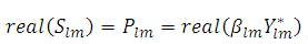
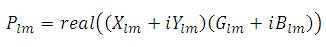
Distribution power flow is used to determine the steady state of bus powers, bus voltages and losses of the system. In the earlier methods of load flow studies only PQ buses are considered and flat voltage profile of all buses is assumed at the starting of the load flow. In this paper a new approach is used for the load flow to determine the steady state voltages and powers of each bus without flat voltage profile. If the system consists of PV buses the same load flow is used by modifying certain equations. As we know the equation for complex power

According to ohms law


If lm is the branch element in the RDS then Eqn(9) is represented as follows
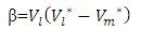
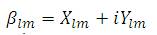
The term  is taken as new variable and represented as β. So the equation for β is represented as
The size of the element incidence matrix is “Nb X Nb.” It is constructed by using the following procedure.
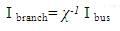
The bus currents are calculated by using Eqn (7)
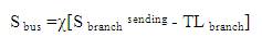
As the transmission losses are ignored for the first iteration and the disparity between the specified powers and the calculated powers are the part of the transmission loss, .TLlm r is the transmission loss part for 'lmth' element for 'rth'iteration.
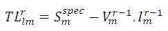

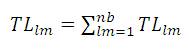
Where 'r' is the iteration count.
The criteria is continuing up to this load flow meeting of the convergence which is the tolerance of 0.0001.
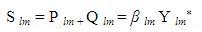
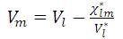
When the power is supplied at multiple ends of the system, other supplying buses except slack bus are treated as voltage controlled buses. Equation (5) is modified for the mth voltage controlled bus
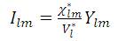
where Xlm is the real value of the βlm
Ylm is the imaginary value of the βlm
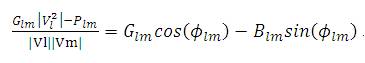
The trigonometric equation is to be solved to get the phase angle φ each PV bus m and the reactive power can be updated as

IEEE 33-bus system is considered to find the optimal location of capacitors PGSA & GA optimization methods. The system has 4 feeders which supply to 33 load centres. The system has 33 buses, 32 lines, 12.66KV as a base voltage and 100MVA as a base MVA as in Figure.1. IEEE 69-bus system is considered to find the optimal location of capacitors PGSA & GA optimization methods. The system has 69 buses, 68 lines. The system has 12.66KV as a base voltage and 100MVA as a base MVA as in Figure 2. V Solution Methodology
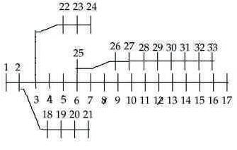
Figure 1. Single line diagram of 33 bus Radial Distribution System
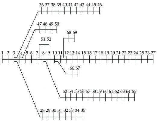
Figure 2. Single Line Diagram of 69 bus Radial Distribution System
The plant growth simulation algorithm[10] is based on the plant growth process, where a plant grows a trunk from its root; some branches will grow from the nodes on the trunk; and then some new branches will grow from the nodes on the branches. Such process is repeated, until a plant is formed. Based on an analogy with the plant growth process, an algorithm can be specified where the system is to be optimized First one of the “grows” begins at the root of a plant and then the second “grows” begins at the branches continually until the optimal solution is found. By simulating the growth process of plant phototropism, a probability model is established. In the model, a function g(Y) is introduced for describing the environment of the node Y on a plant. The smaller the value of g(Y), the better is the environment of the node for growing a new branch. The outline of the model is as follows; A plant grows a trunk M, from its root B0. assuming there are k nodes BM1 , BM2 , Bm ,.....BMk that have been the better environment than the root on the trunk M, which means the function g(Y) of the nodes and satisfies g(BMi) < g(Bo) then morphactin concentrations CM1 ,CM2,….,CMk of nodes BM1 , BM2 , BM3 , …..,BMk are calculated using
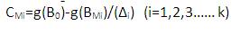
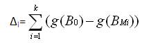
The significance of the above equation (X) is that the morphactin concentration of a node is not only dependent on its environmental information but also depends on the environmental information of the other nodes in the plant, which really describes the relationship between the morphactin concentration and the environment.
A complete algorithm for the proposed method of the capacitor placement is given below[10]:
The genetic algorithm is a global search technique for solving optimization problems, which is based on the theory of natural selection, the process that drives biological evolution. Genetic Algorithm proved to be a very effective and efficient tool for operation and control of the power system. Among the various application schemes GA based control scheme has played a significant role in AGC.
Step 1. Start: Create random population of n Chromosomes
Step 2. Fitness: Evaluate fitness of each chromosome in the population
Step 3. New population
Selection: Based on fitness function
Step 4. Replace: old with new population and the new generation
Test: Test for problem criterion
Loop: Continue step II-V until criterion is satisfied.
The solution methodology is given by following steps
Step 1: Read system data's (Bus data's and Line data's).
Step 2: Calculate the Y-bus and perform the load flow analysis and find out the voltage magnitude and power flow in branches.
Step 3: Performs the TS Initialize Tabu list, Tabu size and initial solution, and find the optimal location of capacitor placements.
Step 4: Place the capacitor at appropriate location which was determined in the previous.
Step 5: Perform the load flow analysis and compare the results before and after placement of capacitors.
The proposed method has been programmed using MATLAB. The effectiveness of the proposed method for loss reduction by capacitor placement is tested on 33 and 69 bus radial distribution systems. The results obtained in the proposed method are explained in the following sections.
The first test case for the proposed method is a 33-bus radial distribution system single line diagram as shown in in Figure 1. The line and load data of the feeders are taken from the reference [12]. The base values of the system are taken as 12.66 kV and 100MVA. Figure 3 shows the flowchart for Capacitor Placement. Tables 1, 2 and Figures 4, 5 depict results of PGSA. The values in Table 5 show the voltage profile values before and after capacitor placement. The values in Table 6 explain the total power loss, total reactive power loss, cost of saving after capacitor placement and elapsed time values. In Figure 8 the Graph shows the comparison of voltage profile values before and after capacitor placement. The red colour curve of the graph shows the voltage profile before the capacitor placement. The blue colour curve of the graph shows the voltage profile after the capacitor placement. In Figure 9 the Graph shows the best cost reduction with respect to the number of iterations. Tables 5, 6 and Figures 8, 9 depict results of GA.
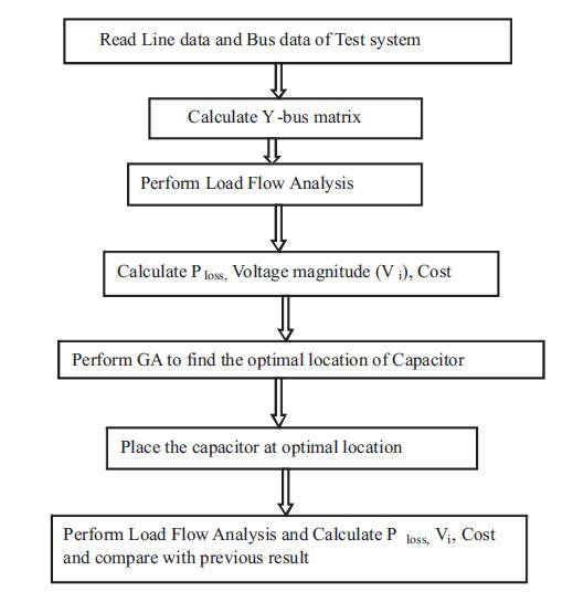
Figure 3. Genetic Flowchart of Solution Algorithm for Capacitor Placement
The next test case for the proposed method is a 69-bus radial distribution system single line diagram is shown in Figure 2. The line data and feeder characteristics are taken from reference [13]. Tables 3, 4 and Figures 6, 7 depict results of PGSA. The values in Table 7 show the voltage profile values before and after capacitor placement. The values in Table 8 explain the total power loss, total reactive power loss, cost of saving after capacitor placement and elapsed time values. In Figure 10 the graph shows the comparison of voltage profile values before and after capacitor placement. The red colour curve of the graph shows the voltage profile before the capacitor placement. The blue colour curve of the graph shows the voltage profile after the capacitor placement. In Figure 11 the graph shows the best cost reduction with respect to number of iterations. Tables 7, 8 and Figures 10, 11 depict results of GA.
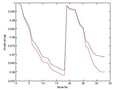
Figure 4. Voltage Profile of 33 Bus System Before and After Compensation
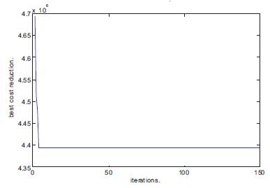
Figure 5. Best Cost Reduction of 33 Bus System
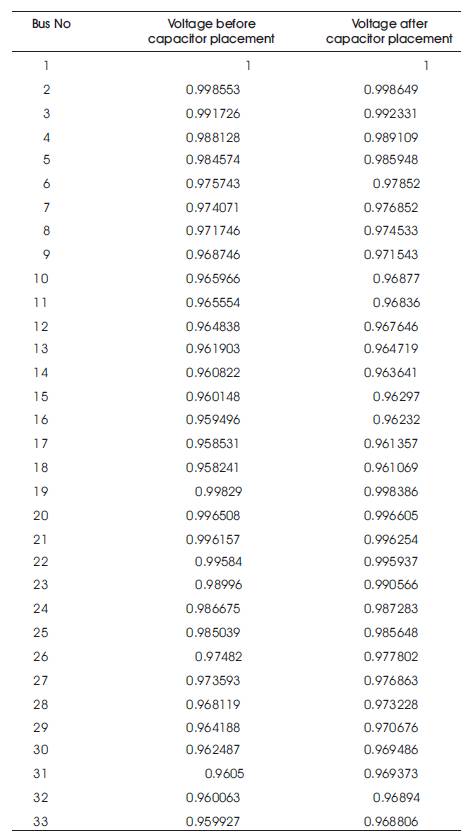
Table 1.Voltage Profile of 33 Bus Radial Distribution System
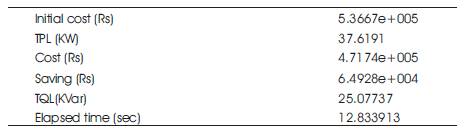
Table 2. Summary of results for 33 bus radial distribution system

Table 3. Voltage profile of 69 Bus Radial Distribution System
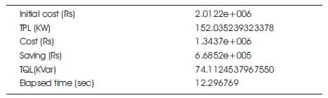
Table 4. Summary of results for 69 Bus Radial Distribution System

Table 5. Voltage profile of 33 Bus Radial Distribution
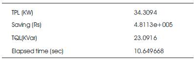
Table 6. Summary of results for 33 Bus Radial Distribution System
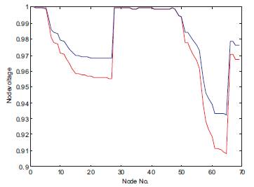
Figure 6. Voltage Profile of 69 Bus System Before and After Compensation
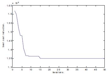
Figure 7. Best Cost Reduction of 69 Bus System

Figure 8. Voltage Profile of 33 Bus System Before and After Compensation

Table 7. Voltage Profile of 69 Bus Radial Distribution System
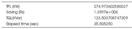
Table 8. Summary of results for 69 Bus Radial Distribution System
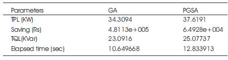
Table 9. Summary of results for 33 Bus Radial Distribution System For PGSA and GA
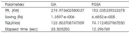
Table 10. Summary of results for 69 Bus Radial Distribution System for PGSA and GA
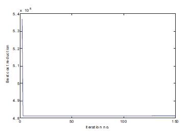
Figure 9. Best cost reduction of 33 Bus System
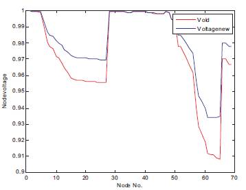
Figure 10. Voltage Profile of 69 Bus System Before and After Compensation
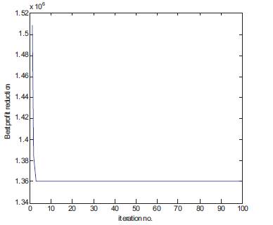
Figure 11. Best Cost Reduction of 69 Bus System
Table 9 shows the values for real power loss, reactive power loss, time for iteration and cost saved after the capacitor placement for both the optimization methods GA and PGSA. For the present case study analysis GA shows the better result compared to PGSA for cost saving in 33 bus radial distribution system. The values in Table 10 show the values for real power loss, reactive power loss, time for iteration and cost saved after the capacitor placement for both of the optimization methods GA and PGSA. For the present case study analysis GA shows the better result when compared to PGSA for cost saving in 69 bus radial distribution system.
This work has been successfully applied in PGSA & GA optimization methods for determining the optimal location of capacitor placement in 33 & 69 bus radial distribution systems for minimum value of objective function. Here the power losses and cost savings are reduced by the placement of capacitors. By placing the capacitor the voltage level can always be in allowable range. So the power losses in the systems are reduced to a great extent by the optimal placement of capacitors in the distribution system.