For optimal distribution network planning, many mathematical models have been proposed in the past for instance, [1, 3, 4, 6] are static models, giving an optimal solution for a fixed set of data and a single time period. Essays in dynamic planning, considering the evolution in power demand through time and consequent topological changes in the networks (new branches, new sub-stations, reinforcements [5], etc.) have never been a definite success, when applied to real sized networks. The mathematical models behind those proposals either were heavy or neglected several project features that engineers take as important on distribution system design; for example, economies gained from cables in the same trench, reuse of disclassified lines, reshaping the whole network by introducing a new substation, etc. Furthermore, the vast majority of the model proposals, on the last 15 years [7], were aimed at a so called “Optimal solution”. However, during the last few years the objective of reaching this optimal concept has been challenged more and more, with the acceptance of principles of the “least cost planning approach [2]. This evolution favors the option for multi-criteria methods and for algorithms giving, as an answer, a large set of possibly good solutions, instead of a single optimum.

Genetic algorithms share precisely this property, and therefore an investigation has been made on their behavior in the distribution network design or Distribution Planning Problem (DPP). This research has been directed into answering the following questions:

• Can genetic algorithms adequately model the DPP problem?
• Is it possible to develop efficient computing algorithms for real size networks?
• Has the genetic approach an easy interface with multi criteria decision making procedures?
• Do genetic algorithms show any advantages over previous proposed approaches?

As the following sections report, the answer is positive to all these four questions. In fact, differently from many models previously proposed, this new model is flexible enough so that many realistic features and conditions of practical nature may be taken care of. For instance: The inclusion of multiple feeders in the same trench, with the related savings achieved;

• The possibility of declassifying lines at some stage, and of re- using them at a later stage;
• The possibility of generating solutions with some open loops, which may be valuable from a reliability point of view;
• Considering multi-objectives;
• Dealing naturally with load diversity factors;
• No need to specify, in advance, at which year a substation should be built or put into service.

The paper is organized as; section-1 reveals about Genetic Algorithm, section-2 reveals about Distribution Planning Model, section-3 explains about Proposed Algorithm, section-4 focus on Case Study.

Genetic Algorithms (GA) are search and optimization methods [8] on natural evolution. They consist on a population of bit strings transformed by three genetic operators: selection, crossover and mutation. Each string (chromosome) represents a possible solution for the problem being optimized and each bit (or group of bits), represents a value for some variable of the problem (gene). These solutions are classified by a evaluation function, giving better values, or fitness, to better solutions. Although there are many forms for Genetic Algorithms, the authors will only refer to the canonical algorithm. This means that they will be dealing with three genetic operators (selection, crossover, and mutation) and linear, binary, fixed–size chromosomes. Canonical GA use a fixed-size, non-overlapping population scheme and each new generation is created by the selection operator and altered by crossover and mutation. The first population is generated at random.

Each chromosome represents a potential solution for the problem to solve and must be expressed in binary form. For instance, if we want to maximize the function f(x) =x², in the integer level I = [0, 31] we could simply code x in binary base, using 5 bits. Each solution must be evaluated by the fitness function to produce a value. For example, the chromosome 11011 would receive the fitness value 27² =729, while the chromosome 00111 would receive the value 7² = 49. The pair (chromosome, fitness) represents an individual [10].

The selection operator creates a new population / generation by selecting individuals from the old population, biased towards the best. This means that there will be more copies of the best individuals, although there may be some copies of the worst. This operator can be implemented in a variety of ways. This implementation is suited to a future distributed implementation and is very simple: every time we want to select an individual for reproduction, we choose two, at random, and the best wins with some fixed probability, typically 0.8. This scheme can be enhanced by using more individuals on the competition or even by considering evolving winning probability.

Crossover is the main genetic operator and consists in swapping chromosome parts between individuals. The simplest crossover operator is implemented by selecting a random cross over point in chromosome and swapping the genes that reside between the crossover point and end of the chromosome. For example if we have two individuals:

A = 010100 ; B = 010111

And choose a crossover point C=3 (indicates by 'I') the resulting individuals after crossover would be

A' = 010111 ; B' = 010100

Crossover is not performed open every pair of individuals, its frequency being controlled by a crossover probability. This probability should have a large value, typically P_c = 0.8.

The last genetic operator is mutation and consists in toggling a random bit in an individual. The operator should be used with some care, with low probability, typically P_m = 0.001, for normal populations.

A canonical GA is a very simple process: we first generate a random initial population, evaluate it and start creating new populations by applying genetic operators.

Obviously, there is the need for some book keeping functions, for statistics and so on, but they are not central to this explanation.

This is very simple behavior hides a powerful processing done by GA. In fact, the combination of selection and crossover leads to a proliferation of individual that possess small, tightly coupled blocks of bits leading to good performance. These blocks, usually called schemata, are replicated through selection and combined or separated by crossover, and mutation works as a kind of “life insurance”. Some important bit values (genes) may be lost during selection; mutation can bring them back. if necessary. Nevertheless, too much mutation can be harmful: a mutation probability of 0.5 always leads to random search, independently of crossover probability.

So, GA tends to select individuals with good performance and recombine some of their building blocks, creating more and more copies of good schemata, simply by the use of selection and crossover. This hidden processing is called implicit parallelism because the number of schemata processed in each generation is typically O (N³), being N the population size. This compares very well with the number of fitness function evaluations, N. This characteristics is distinctive of Genetic Algorithms.

This section presents a model to solve the problem of the optimal sizing, timing and location of distribution substation and feeder expansion, using genetic algorithm. The model allows the inclusion of constraints related to network radiallity, voltage drops [11] and reliability assessment [16].

The objectives for distribution system planning that will be discussed are related to providing the designs and associated implemented plans necessary for an orderly expansion of facilities, minimizing new facility installation costs and operation costs, as well as acceptable level of reliability, under the following constraints [15] :

• Operating of the networks under radial configuration (although some open loops may exists);
• Voltage drop constraints;
• Power demand specifications;
• Possible site location for substation and lines prespecified.

Facility installation costs will be divided in three elements: substation capacity expansion cost and new feeder cost. Power losses in the network will be taken is operated costs [14]. Already existing elements (substation or feeder) are included at no investment cost in the model; however, their power losses are estimated and taken in account [12-13].

The following assumptions are made:

• A peak load is considered for each expansion planning (load forecasting is out of the scope of this paper).some extra information about load curves (such as load factor) is required, in order to evaluate losses and assess reliability indices such as average load disconnected or average annual energy not supplied.
• New installation facility candidates are known beforehand, and their location and installation costs estimated.

An expansion strategy will be driven by load growth. The planning will be divided into several stages (one year, for instance). One aims at having, as result, a list of investments to be made at each stage.

The genetic algorithm approach to the DPP is drawn under the following general lines:

• A set of variables is chosen to represent a multi-stage network solution; these variables are encoded in a chromosome.
• A genetic algorithm is applied to a family of solutions, giving birth to new generations.
• Each solution in the new generation is evaluated through a fitness function, that includes investment costs, power loss costs, reliability, voltage drop deviations; non compliance with other constraints is dealt with by the fitness function - an unfeasible solution, with by the fitness function - an unfeasible solution, with a low fitness value, will hardly survive.
• At the end of the process, a family of well fitted plans is available.

For a m-stage planning problem, the following (0-1) Integer decision variables could be defined:

F_is : F_is = 1 : if feeder i is used at stage s
  F_is = 0 : otherwise 
S_is : S_is = 1 : if substation i is used at stage s 
S_is = 0 : otherwise 
E_is : E_is = 1 : if subst. expansion i is used at stage
E_is = 0 : otherwise

Existing Facilities may be considered by fixing their expective values to 1.

The direct coding of the above variables into a chromosome has been tried and tested. Although the results obtained were satisfactory, the process was not very efficient, because the extremely large number of unfeasible solutions appearing at each generation led to a large computing time before reaching an acceptable stability.

Therefore, the authors devised a new coding process. Its requirements were: it should lead to a minimum amount of unfeasible solutions generated; and it should provide very fast decoding, as this operation is required at every fitness evaluation. Its characteristics are:

• At one time stage, some nodes might be assigned with load values, while other may have a forecasted Zero load.
• A node with a positive load must be connected to, at least one feeder, while nodes with Zero load may either have no connections or have one or more connections in order to allow power flow to other nodes.
• Each node is represented in the chromosome by a number of bits needed to encode the number of possible connections to it e.g., if four lines connect to the node, one needs two bits, if it is a positive load node, or a three bit string, if it is a zero load node ( to include the case where no line goes through that node).
• A substation is assumed as a special type of line, that may be connected to the nodes chosen as possible building sites.

This encoding strategy is such that it gives, as result, only solutions with a number of lines = (nodes-1), a radiallity condition.

A few other details were included in the model, which are not relevant to its understanding but helped in gaining computer efficiency.

The fitness function must reflect both the desired and the unwanted properties of a solution, rewarding the former and strongly penalizing the latter. In the DPP, desired properties are, for instance, low cost and high reliability, while unwanted features are non-radial configurations (open loops are accepted, but not closed loops), violations of thermal cable limits or of voltage drop constraints.

Fitness is evaluated a posteriori; therefore it may be nonlinear, non-continuous, non-convex, whatever. This is very advantageous over strict mathematical programming approaches.

The general trend is to maximize fitness. Figure 1 presents the general scheme of evaluation of the fitness of a solution, represented by a chromosome, at any generation. The function g (x_i), h(x_k) and v(x_k), referred to in this Figure, must be chosen so that, for no matter what solutions x are evaluated, one always obtains

(1)

From the equation (1) the function, have included the following:

• Investment costs IC are added for all the planning stages, considering a fixed discount rate;
• Power loss costs PL are treated in the same way;
• Voltage quality VQ may be assessed in many ways - we have used the following scheme:
  • If the voltage drop at any node exceeds some threshold(e.g.,8%), the solution has been taken as unfeasible and its fitness evaluated by function
  • Else, if the voltage drops at some nodes lie within a given interval (e.g. 5% to 8%), the voltage quality index of the solution is assessed by the sum of the square deviations to the lower limit of this interval
  • Else, if at all nodes the voltage drop stays below that lower limit, the voltage quality index receives 0 value.

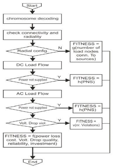
Figure 1. Fitness Function Evaluation Scheme

From the equation (2) the reliability (RB) of a solution is evaluated through the approximate calculation of the expected annual energy not supplied this calculation takes into account the existence of open loops in the network; we have used the following scheme:

An upper bound U_r in reliability level is calculated assuming that no switching devices are included in the network - therefore, disconnections take place only at the substation.

A lower bound Lr is calculated assuming that all branches are equipped with switching devices allowing the isolation of failed branches and service restoration (taking in account the line capacities).

Reliability fitness is given by

(2)

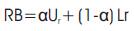
Where α Є [0, 1] is an “improvement coefficient” that aims at simulating the effect of a compromise solution in switching device location policy as this, in itself, is a very complex problem.

The fitness value f of a solution x is given by:

(3)

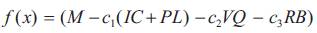
Where, M-large (enough) constant value;
C₁ - constants externally fixed.

Other special features:

• The DC load flow calculations are used as a first filter for un feasibilities, and are performed at the same time as the structure of the network is recognized - this strategy proved very efficient;
• For AC load flow calculations, we used the method described in [17], applied to balanced systems, as it was specially developed for radial networks;
• Before load flow calculations, load values to be used may be affected by coefficients to tale in account the diversity in demand load curves - this feature also distinguishes this GA approach from other models.

The GA approach was applied to the system shown in Figure 2, where solid lines represent existing cables in the initial radial system, and dotted lines represent possible sites for the expansion of the system. A complete data listing may be obtained from the authors, by request. The proposed substation sizes and other complementary system data are shown below

Number of time stages 2(+initial)
Discount rate 10%
Nominal voltage 15kV
Voltage thresholds 5%,8%
No. of nodes 3 X 50
No. of branches total 3 X 64
No. of potential branches 3 X 48
Total load for each time stg. (MVA) 45; 63; 79.5
Feeder cost (PTE) 4 X 10⁶ / km

Let us assume each substation having a capacity of 100MVA and each node having a uniform loading of 7MVA.

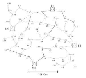
Figure 2. Original Test System

By considering Figure 2 as reference the load distribution has been modified as shown in Figure 3,

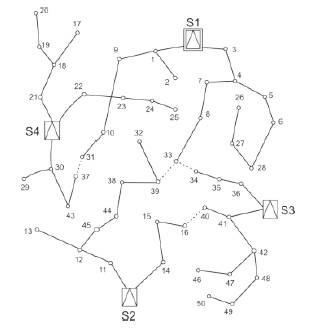
Figure 3. Modified System

But in Figure 3 the load distribution has become inefficient due to over load on substation S₁.

Though more load has become burden on the first substation S₁, to compensate or to reduce the burden on the substation S₁, the loads are distributed or modified as shown in Figure 4.

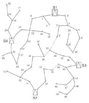
Figure 4. Optimal System

In Figure 4, load 33 is connected to substation S₃ and thus the load on the S₁ has reduced.

Let each substation capacity is of 100MVA.

Before modification as per Figure 3.

Each load on substation is 7% of substation capacity (100 MVA).

Number of loads on each substation
S₁ - 15 105 MVA (over loaded) 
S₂ - 11 077 MVA 
S₃ – 11 077 MVA
S₄ - 13 091 MVA

An attempt has been made in this research work strongly to compare and discuss the results of proposed case study with V. Miranda et al [18]. The Table 1 shows the load on sub station and Table 2 shows the total number of load, connected to sub-station before and after the proposed genetic algorithm.

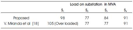
Table 1. Results comparison

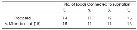
Table 2. Number of Loads Connected to Substation

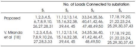
Table 3. Number of loads on each substation

The Tables 1, 2 and 3 also reveals the comparison results of the proposed algorithm with the results of V. Miranda et al [18], the percentage of load on substations S₁, S₂, S₃, S₄ are 105,77,77,91, respectively as per the results of V. Miranda et al [18] where as the percentage of load on substations S₁, S₂, S₃, S₄ are 98, 77, 84, 91, respectively by the proposed algorithm. Hence, the over load on substation S₁ has been eliminated.

Hence, the over load on substation S₁ has been reduced from 105% to 98%.

Figure 4 shows the final configuration which is an alternative with less investment and more reliable.

The work presented in this paper clearly demonstrates that a GA approach to a multi-stage distribution system planning problem is feasible and advantageous; it provides the planner with a set of time-ordered investment decisions which is not obtained from static sub-optimizations, but directly from the consideration of the time dimension of the problem. In this respect, it is more complete, which claim feasibility under constrained computing environments. The results of GA are a generation of solutions, filtered through the struggle for survival. Therefore many interesting and valuable exercises on comparisons and trade offs may be executed, helping the planner to gain insight on the problems faced with and allowing field for better decisions to be taken.

The fact that many solutions will be available also enhances the opportunity for multi criteria methods to be explicitly applied.

The authors would like to express their profound gratitude to the Principal and the Management of ACE Engineering College and friends who have directly or indirectly helped in this paper.