The HVDC transmission system is becoming ever more complex, further, demand for reliable supply of electricity is growing, increasing the need for a higher level of system reliability. A probable solution might be to incorporate controllable power components within the system. One such important thing is smoothing reactor or DC reactor. In this paper the effect of failure rate and repair time on expected capacity level or power transmission capacity of smoothing reactor at different inductance values with one, two and without spares is analyzed and compared. And also effect of number of spares on expected capacity level is presented.
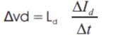
Protection of HVDC systems may be divided into four categories; over voltage protection, over current protection, damper circuits and DC reactors [7,6]. DC reactors prevent the commutation failures in the inverter by limiting the rate of increase of direct current during the commutation in one bridge when the direct voltage of another bridge collapses [1,8]. Practically speaking DC reactor is always required, and its inductance is the principal factor limiting the rate of rise of direct current and improves the expected capacity or power transmission capacity level of reactor[4]. The magnitude of rise of current during commutation depends on the overlap time (for HVDC 80).
Generally DC reactor in HVDC system having inductances of 0.4H to 1.0H is connected in series with each pole of each converter station [5].
Availability or reliability can however be improved by reducing the failure rates and the mean time to repair of the equipment associated with DC systems and by utilizing appropriate redundancy measures in key areas [2,5].
A DC system is composed of many individual components. Some components of a DC system such as filters, transformers and smoothing reactors, require special modeling techniques[3].
In this paper, Markov models for smoothing reactor at different inductance values at different failure rates and repair times with and without spares are presented.
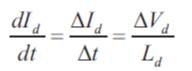
All inverter faults lead to the collapse of the direct voltage of a bridge. This voltage remains at zero for about 3/8 of a cycle, which is several times greater than the time available for commutation. The counter voltage of the affected inverter pole falls to ½ (half) times from the normal value. Consequently, the direct current through the inverter rises, tending toward a new steady value such that the new IR (resistance) drop in the line is difference between rectifier voltage and the reduced inverter voltage. The rise of current prolongs commutation and, if excessive, causes commutation failure which, in turn, leads to an additional large decrease of inverter voltage which further increases the rise of direct current. Thus the failure is likely to spread to all the bridges of the affected pole, decreasing the expected capacity level (or) power transmitted by the DC line to half of its pre fault value. The rate of rise of current is limited by adding smoothing reactor in series to the HVDC system.
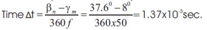
No. of bridges per pole = 2
Rated voltage per bridge = 200kv
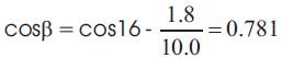
Rated Current = 1.8kA
Greatest permissible current at the end of commutation = 10.0kA
Frequency = 50hz
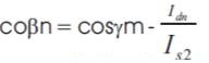
βn = normal ignition advance angle
At different inductor values different reactor ratings are tabulated in Table 1.
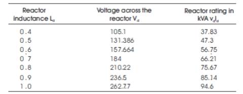
Table 1. The Effect of Reactor Inductance Values on Reactor Rating
In this paper, Markov modeling approach is used to account the distribution of component failure over time. It is possible to compute the reliability parameters as the long term probability of the system being in a given state by solving a linear differential equation system. The graphical model constructed to display all possible transition paths between states is called state space diagram.
A Markov model can be applied to systems whose random behavior varies either discretely or continuously with time. In this paper Markov modeling has been adapted. Figure 1 shows a basic example of Markov process in a state space transition diagram.
L: failure rate f/yr
M: repair time r/yr
In Figure1 there are states up state (state 1) and down state (state 2). There are two transitions associated with each component, the first representing the failure process and the second representing the repair process. This model implies that the component becomes operational and in service immediately following the repair action. The duration of the failure is limited to the time it takes to install the spare unit rather than to repair the equipment itself.
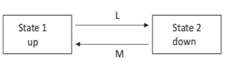
Figure 1. State Space Diagram of two State Markov Process
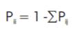
In this paper, only the equations for calculating the steady state solution of the system are presented. This solution gives the probability of being in a certain state after an infinite time in the system. It can be shown that this steady state solution can be found by solving the eqn1.

Here Pi is the steady state probability of system or element being in the ith state.
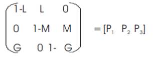
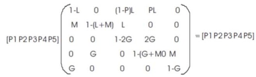
Q = State Transition Probability Matrix for the Markov Process is
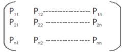
In this matrix Pij is the transition rate from state i to state j. The diagonal element Pij are defined in the eqn 3
Consider the state space diagram of smoothing reactor belonging to bipole HVDC system without backup as shown in Figure 2.
In Figure 2 State 1 represents up state. State 2 and 3 represents down states.
L: failure rate f/yr
M: repair time r/yr
G: installation time ins/yr
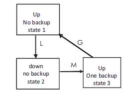
Figure 2. State Space Diagram of Smoothing Reactor Without Back Up
The limiting state probabilities of above system can be determined as follows.
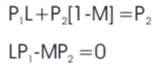
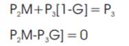
| P11 = 1-L | P12 = L | P13 =0, | P21 = 0 |
| P22 = 1-M | P23 = M, | P31 = G | P32 = 0 | P33 =1-G |
Where P11 = probability of system or element being in state 1 after completion of first interval
By using STPM approach
[ P1 P2 P3 ]
From the eqn, 4
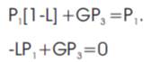
Arranging eqns 6,7 and 8 in matrix form
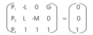
Applying Cramer's rule to the above,
eqn 9 obtained with limiting state probabilities for failure rate 0.2 f/yr, repair time 100 days, installation time 2 days or 48 hours are
For selected values of failure rates and repair time (EEL river DC system) expected capacity level or power transmission capacity of smoothing reactor at different inductance values is evaluated and tabulated in Table 2 and 3 respectively.
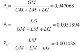
Consider now the situation that could exist it one spare was normally available. In this case, When a reactor fails, it can be replaced by the spare reactor. Provided that either the spare has not already been used or the component it has replaced has been repaired and is available as a spare. This provides the state space model of smoothing reactor with one backup is shown in Figure.3. using STPM approach
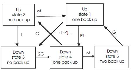
Figure 3. State Space Diagram of Smoothing Reactor with one Backup
Let P be the probability that back up element is available.
State 1 represents the state in which reactor is operatable. When failure occurs, the probability of going to state 4 is PL and the probability of going to state 3 is (1-P)L.
P= probability that the backup element is available
=Mb / (Lb+Mb) Using STPM approach
Where,
Mb = repair time of backup element
Lb = failure rate of backup element
Solving the eqn 10, the state probabilities of Figure 3 can be calculated by using limiting state probability approach. In Figure 3 both state 1 and 2 represent operable conditions and can be combined to create a single up state with probability of P1 +P2 .
For selected values of failure rates and repair times(EEL River DC system) expected capacity level or power transmission capacity of smoothing reactor at different inductance values is evaluated and tabulated in Table 4 and Table 5 respectively
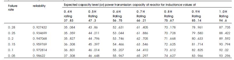
Table 2. Effect of Failure Rate on Expected Capacity Level or Power Transmission Capacity of Smoothing Reactor Without Backup
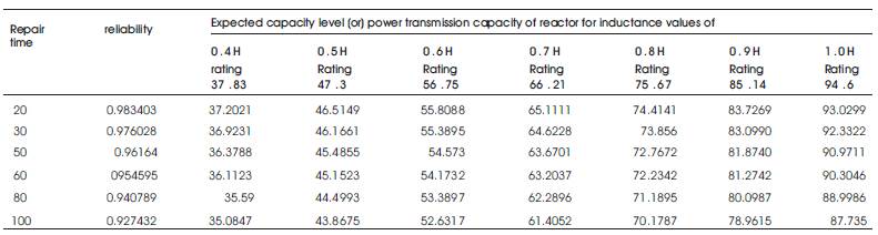
Table3. Effect of Repair Time on Expected Capacity Level or Power Transmission Capacity of Smoothing Reactor Without Backup
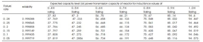
Table 4. Effect Of Failure Rate on Expected Capacity Level or Power Transmission Capacity of Smoothing Reactor With one Backup
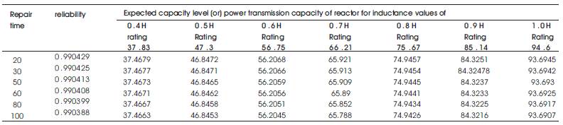
Table 5. Effect of Repair Time on Expected Capacity Level or Power Transmission Capacity of Smoothing Reactor With One Backup
State space diagram of rector with two backups is as shown in Figure 4. Using STPM approach limiting state probabilities is evaluated. For selected Failure rates and repair times expected capacity level or power transmission capacity of smoothing reactor with two backups is tabulated in Table 6 and Table 7 respectively.
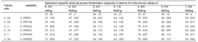
Table 6. Effect of Failure Rate on Expected Capacity Level or Power Transmission Capacity of Smoothing Reactor With Two Backups
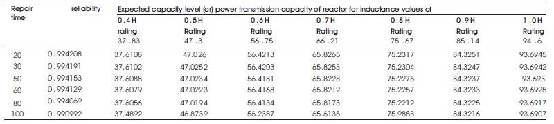
Table 7. Effect of Repair Time on Expected Capacity Level or Power Transmission Capacity of Smoothing Reactor With Two Backups
Tables 2, 4 and 6 represent variation in expected capacity level without, with one and with two backups due to variation in failure rate. In Table 2, 4 and 6 different inductance values are taken in First column; in second column respected reliability values are taken. Remaining columns (3, 4…9) represent expected capacity level of reactor at different reactor ratings.
Tables 3, 5 and 7 represent variation in expected capacity level with out, with one and with two backups due to variation in repair time. In Table 3, 5 and 7 different inductance values are taken in first column; in second column respected reliability values are taken. Remaining columns (3, 4…9) represents expected capacity level of reactor at different reactor ratings. Table 8 gives expected capacity level of reactor with and without backups at different reactor inductance values at failure rate of 0.28f/yr. In this table different inductance values are taken from 0.4H to 1.0H in first column. In second, third and fourth columns expected capacity levels without, with one and two backups are taken.
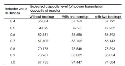
Table 8. Effect of Reactor Inductance Values on Expected Capacity Level or Power Transmission Capacity of Smoothing Reactor
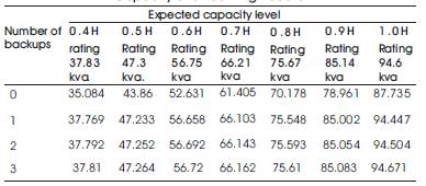
Table 9. Effect of Number of Backups on Expected Capacity Level or Power Transmission Capacity of Smoothing Reactor
Figure 5, 7 and 9 shows the effect of (or) variation in expected capacity level or power transmission capacity level of smoothing reactor without backup and with one and two backups respectively. Here expected capacity level of reactor is evaluated at different failure rates. In figures 5, 7 and 9 curve 1 represents the variation in power transmission capacity level due to increase in failure rate at inductance value of 0.4H. Similarly curve 2, 3,4,5,6 and 7 are at inductance values of 0.5H, 0.6H, 0.7H, 0.8H, 0.9H and 1.0H respectively.
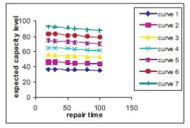
Figure 5. The Effect of Failure Rate on Expected Capacity Level of Reactor Without Back Up
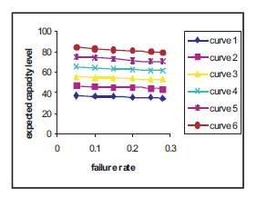
Figure 6. The effect of repair time on expected capacity level of reactor without back up
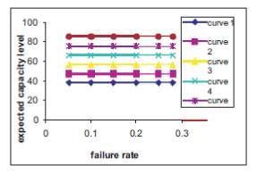
Figure 7. The Effect of Failure Rate on Expected Capacity Level of Reactor With one Backup
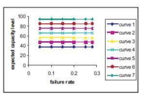
Figure 8. The Effect of Repair Time on Expected Capacity Level of Reactor With one Back Up
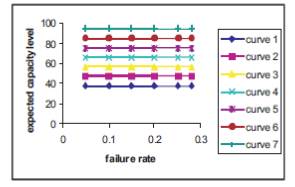
Figure 9. The Effect of Failure Rate on Expected Capacity Level of Reactor With Two Backups
Figures 6,8 and 10 show the effect of (or) variation in expected capacity level or power transmission capacity level of smoothing reactor without backup and with one and two backups respectively. Here expected capacity level of reactor is evaluated at different repair times. In Figures 6, 8 and 10 curve 1 represents the variation in power transmission capacity level due to increase in repair time at inductance value of 0.4H. Similarly curve 2, 3,4,5,6 and 7 are at inductance values of 0.5H, 0.6H, 0.7H, 0.8H, 0.9H and 1.0H respectively.
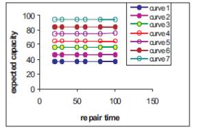
Figure 10. The Effect of Repair Time on Expected Capacity Level of Reactor With Two Backups
In Figure 11, reactor inductance values are taken on x-axis and expected capacity level is taken on y-axis. Curve 1 represents expected capacity level without backup. Curve 2 and curve 3 represents expected capacity level with one and two backups.
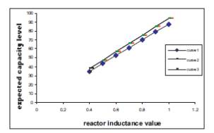
Figure 11. The Effect of Reactor Inductance Value on Expected Capacity Level
In Figure 12 number of backups 1, 2, 3 and zero are taken on x-axis and expected capacity level at different ratings are taken on y-axis. From this increase in number of backups increases the expected capacity level of reactor.
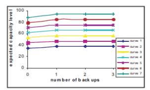
Figure 12. The Effect of Number of Backups on Expected Capacity Level of Reactor
The following are the conclusions drawn from the present work.