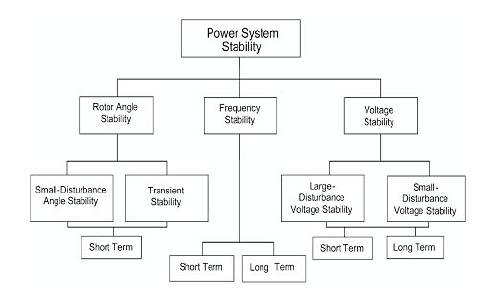
Figure 1. Classification of Power System Stability
This paper presents a simple method of evaluating the first swing stability of a large power system in the presence of Unified Power Flow Controller (UPFC) device. First a UPFC and the associated transmission line are considered and represented by an equivalent π–circuit model. The above model is then interfaced to the power network to obtain the system reduced admittance matrix which is needed to generate the machine swing curves. The above π –circuit model can also be used to represent other FACTS devices (SSSC and STATCOM) by selecting appropriate values of control parameters of the UPFC. The complex voltage at two end buses of the π-circuit model is also evaluated during simulation to implement various existing control strategies of FACTS devices and to update the reduced admittance matrix. The effectiveness of the proposed method of generating dynamic response and hence evaluating first swing stability of a power system in the presence of UPFC device will be tested on the ten-machine New England system.
Evaluation of first swing stability (FSS) limit is one of the important aspects in power system planning and operation studies. A first swing stable system may be considered as stable if the system has adequate damping[1]. Lack of adequate damping may cause growing oscillations and ultimately the system may become unstable. The FSS limit can be improved by controlling the output power of the severely disturbed machine(s) during transient period[2]. Flexible ac transmission system (FACTS) devices placed at strategic locations are found to be very effective in addressing the above issue. There are various forms of FACTS devices such as SSSC, STATCOM and UPFC. Some of which are connected in series with a line and the others connected in shunt or a combination of series and shunt.
Transient stability is the main factor that limits the power transfer capability of long distance transmission lines. Power utilities are now placing more emphasis on improving the transient stability, especially the first swing stability limit to increase the utilization of existing transmission facilities, [3].
“Power system stability is the ability of an electric power system for a given initial operating condition, to regain a state of operating equilibrium after being subjected to a physical disturbance with most system variables bounded so that practically the entire system remains intact.”
The power system is a highly nonlinear system that operates in a constantly changing environment; loads, generator outputs and key operating parameters change continually. When subjected to a disturbance, the stability of the system depends on the initial operating condition as well as the nature of the disturbance.
The classification of power system stability (Figure 1) is based on the following considerations:
Figure 1. Classification of Power System Stability
Rotor angle stability refers to “the ability of synchronous machines of an interconnected power system to remain in synchronism after being subjected to a large disturbance”. It depends on the ability to maintain/restore equilibrium between electromagnetic torque and mechanical torque of each synchronous machine in the system. Instability that may result occurs in the form of increasing angular swings of some generators leading to their loss of synchronism with other generators.
Voltage stability refers to “the ability of a power system to maintain steady voltages at all buses in the system after being subjected to a large disturbance from a given initial operating condition”. It depends on the ability to maintain or restore equilibrium between load demand and load supply from the power system. Instability that may result occurs in the form of a progressive fall or rise of voltages of some buses. A possible outcome of voltage instability is loss of load in an area or tripping of transmission lines and other elements by their protective systems leading to cascading outages. Loss of synchronism of some generators may result from these outages or from operating conditions that violate field current limit.
Frequency stability refers to “the ability of a power system to maintain steady frequency following a severe system upset resulting in a significant imbalance between generation and load”. It depends on the ability to maintain or restore equilibrium between system generation and load, with minimum unintentional loss of load. Instability that may result occurs in the form of sustained frequency swings leading to tripping of generating units and/or loads.
“A power system can be considered as first swing stable if the post-fault angle of all machines in center of angle (COA) reference frames increases (decreases) until a peak (valley) is reached when the angle starts returning[5]”. In an unstable situation, the angle of one or more generators will monotonically increase (decrease).
Mathematically, a system can be considered to be first swing stable if the following condition holds:

Where,
ti - Is the time at which the rotor angle of generator I reaches the peak
ε - Is a small positive number.
If a system is first swing stable, it is expected that the system damping, governor, etc. usually help to damp oscillations in the subsequent swings.
A unified power flow controller (UPFC) is a member of FACTS family which is connected to a power system in series and shunt combination. It consists of two voltage source converters (series and shunt) coupled through a common dc link as shown in Figure 2.
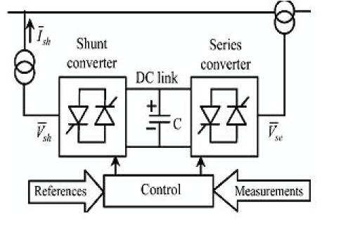
Figure 2. UPFC Schematic Diagram
The dc link provides a path of active power exchange between the converters. Both the series and shunt converters are capable of generating or absorbing reactive power independently. When the shunt converter is kept inactive, the series converter can exchange reactive power with the system and is called a static synchronous series compensator (SSSC). On the other hand, when the series converter is kept inactive, the shunt converter can operate as a static compensator (STATCOM) and exchange reactive power with the system. In other words, a UPFC is a versatile FACTS device that can also be used as an SSSC or a STATCOM.
In the case of a UPFC, the controller ultimately produces a series injected voltage ( ) and a shunt injected current (
 ) and which are to be interfaced to the power network as shown in Figure 3. The above Figure 3 can also be used to represent other FACTS devices (SSSC and STATCOM) by selecting proper values of and
  .
.
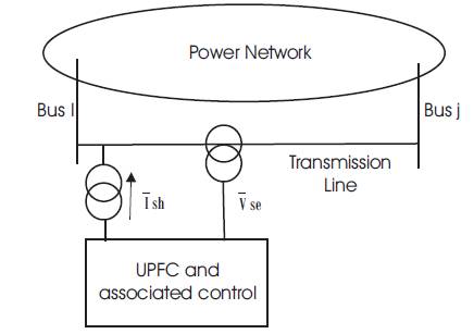
Figure 3. UPFC Interfaced to Power Network
For any system, a general interfacing technique of FACTS devices to power network is not needed to evaluate the system response. However, in power system planning and operation studies, it is necessary to investigate the dynamic performance of a realistic size power system for a large number of contingencies. For such a case, a general technique of interfacing various FACTS devices to a large power network is very essential to efficiently generate the system dynamic responses and that motivates the author to conduct this study. Results of such investigations may be used for screening purpose to identify the critical cases that require further detailed analysis.
This section describes the machine dynamic equations and a simple π-circuit model of a UPFC and other FACTS devices. A technique of interfacing the above π-circuit model to a general power network is also described.
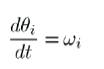
Consider an -machine power system. In general, the classical model of a power system is used to investigate the FSS of the system. In this model, the dynamics of ith machine in the center of angle (COA) reference frame can be represented by the following differential equations.
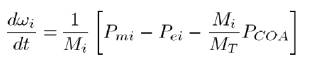
Where,
Here
Where,
θi - Angle,
ωi - Angular Velocity,
Ei' - Internal Voltage Magnitude,
Pmi - Input Mechanical Power,
Pei - Output Electrical Power,
Mi - Moment Of Inertia and
 -Reduced Admittance Matrix of Ith machine
The above equations are very commonly used to generate the dynamic response of a power system without any FACTS device. One of the objectives of this study is to evaluate  by properly interfacing various FACTS devices to the power network so that the conventional technique can be used in generating the system response in the presence of FACTS devices.
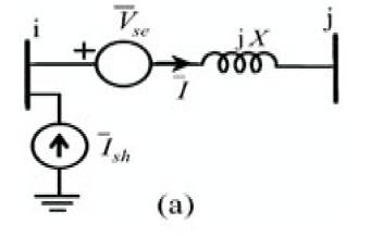
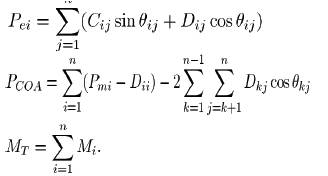
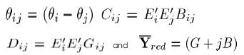
Figure 4a. UPFC is represented by  &
&
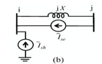
Figure 4b. UPFC is represented by &
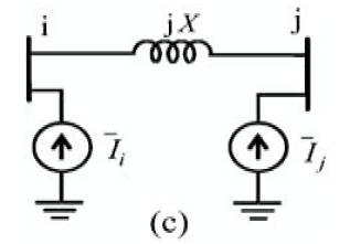
Figure 4c. UPFC is represented by  and
and 
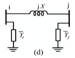
Figure 4d. UPFC is represented by and
and 
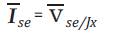
In above Figure 4 (a) the UPFC is represented by a series voltage source and a shunt current source . This represents the dynamic model of a UPFC. For simplicity, the line is first represented by only its series reactance X. The leakage reactance of the series injection transformer (if any) can be included in X. The voltage source in series with X can be represented by a current source in parallel with X as shown in Figure 4 (b).
Where,
Without loss of generality, the current source between buses i and j can be replaced by two shunt current sources (at buses i and j). Such an equivalent circuit is shown in Figure 4 ( c ).
Where,
The shunt current source is replaced by complex power injection and is called the injection model of a UPFC. Such a model is very useful for power flow analysis. However, in this study, the shunt current sources are replaced by shunt admittances( and ) as shown in Figure 4 (d).
Where,
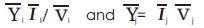
Figure 4 (d) represents the π-circuit model of a UPFC and its associated transmission line. Note that the shunt admittances and are not constant but depend on and and hence the control strategy used.
In Figure 4 (a), the active power (Psc) absorbed by the series converter or can be written as
Here,
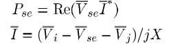
 and
and  are the complex voltage of buses and , respectively.
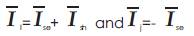
The shunt injected current can be split into two components:  and
and 
supports the active power exchange between the series and shunt converters and it can be written as
Here
δi is the angle of
Here
δi is the angle of
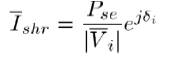
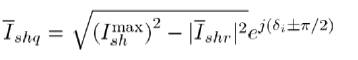
exchanges reactive power with the system. For a given current rating  of the shunt converter , can be written as
As mentioned earlier, the UPFC model can also be used to represent an SSSC or a STATCOM by selecting appropriate values of  and . For an SSSC, it is necessary to set
  and thus
  simply becomes . In this case, is kept in quadrature with the prevailing line current
  . However, for a STATCOM, (and hence ) is to be set to zero. Thus both
  and are also zero. In this case,shr is also zero and thus is the same as .
In Figure 4, it is assumed that the resistance (R) and capacitance (C) of the line are negligible. However, to get more accurate results, it is necessary to include R and C of the line. A technique of incorporating the above line parameters, without modifying the proposed π-circuit mode of Figure 4 (d), is discussed in the following.
The UPFC and the nominal π-circuit model of the associated transmission line (including R and C) are shown in Figure 5 (a). Assume that transferring the line shunt admittance  from right side of to its left side (at bus i) would not make any significant error. Such an equivalent circuit is shown in Figure 5 (b) where a fictitious bus j' is added to split the line reactance X into two components using a constant k(<1). The dotted portion of Figure 5 (b) is exactly the same as Figure 4 (a) and which can ultimately be converted to the proposed π-circuit model of Figure 4 (d). The rest part of Figure 5 (b) can easily be included into the power network of Figure 3. The above technique intelligently incorporates the resistance and capacitance of the UPFC line without practically including them into the π-circuit model.
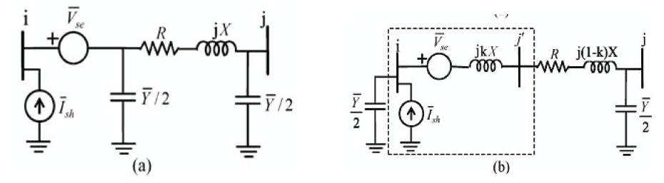
Figure 5. UPFC and the nominal π-circuit model
Consider that a UPFC is placed in one of the transmission lines connected between buses i and j of a general power system as shown in Figure 6(a). The objective is to find the overall reduced admittance matrix (with the UPFC) red and is needed in evaluating the dynamic equations (1) and (2). First replace the loads by constant shunt admittances and then eliminate all physical buses of the system except the UPFC end buses (i and j). The partially reduced system consists of only machine internal buses and two physical buses (i and j) as shown in Figure6 (b). The corresponding partially reduced admittance matrix is represented by  and thus
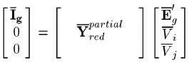
Here
 and
and  are the vectors of generator complex internal g g voltage and current, respectively.
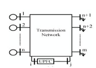
Figure 6(a). Reduced transmission line network after UPFC placed

Figure 6(b). Reduced transmission line network after UPFC placed
The UPFC and the associated transmission line are now replaced by the proposed π-circuit model (Figure 4 (d)) and is shown in Figure 6 (c). For a given operating condition of the UPFC, the shunt admittances of the π- circuit model can be incorporated into the ith and jth diagonal elements of . Afterward, buses i and j can also be eliminated to obtain red as shown in Figure 6 (d).
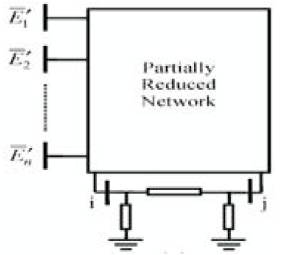
Figure 6(c). Reduced transmission line network after UPFC placed
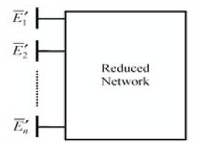
Figure 6(d). Reduced transmission line network after UPFC placed
Then, the system equation becomes
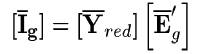
When R and C of the line are considered, it is necessary to Include /2, R and j (1-k) X of Figure 5 (b) into the power network before obtaining . In this case, it is also necessary to replace bus j' by j and reactance kX by X in order to compare the dotted portion of Figure 5 (b) with Figure 4 (a).
The above technique of interfacing the π-circuit model of a UPFC to a power network is also applicable for other FACTS devices (SSSC and STATCOM).
In case of multiple FACTS devices, the two end buses of each device are to be retained in. After incorporating the respective π-circuit model into the end buses are to be eliminated to get that consists of only machine internal buses.
Note that during transient period, the shunt admittances of the π-circuit model are not constant but depend on and which in turn depend on the control strategy used. Thus, is to be updated in each integration step.
1. Read line data, bus data, and generator data
2. Form admittance matrix (Ybus)
3. Perform load flow solution using NR-method
4. Convert the loads to equivalent admittance using YL = (PL-jQL)/VL2
5. Calculate the internal bus voltages of the generator using ELδ'= (V+Qxd'/V)+j(Pxd'/V) and the initial generator angle δ0 = δ'+α
6. Reduce the Ybus matrix to generator internal buses Ybusred = Ynn –Ynr Yrr-1 Yrn.
7. Calculate Pm.
8. Create a fault at any bus and enter the fault clearing time. Find Ybus and Ybusred and output power and angles during fault and after clearing fault.
9. Enter the time of study and calculate phase angle difference of each machine with respect to slack bus.
10. Draw the swing curves.
The single line diagram of 10 machine, 39 bus New England System is shown in Figure 7. First a three-phase fault near bus 26 cleared by opening the line 26–29 is considered.
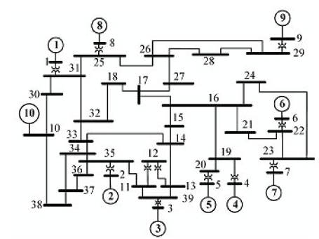
Figure 7. Single line diagram of the New England system
The critical clearing time (CCT) of the fault, without any FACTS device, is found as 80ms. A UPFC is then placed in line 26 – 28 near bus 28 and as a result the CCT is increased to 134ms.
Figure 8 shows the swing curves of all machines of the New England system for a critically stable situation (tc1=134ms) with UPFC.
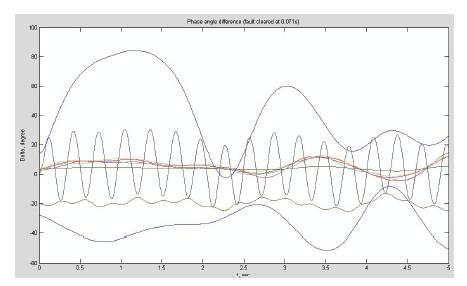
Figure 8. Swing Curves of all Machines of the New England System
The transient stability assessment of 10-machine 39 bus New England System is carried out for the three phase fault of self clearing type. A simple and general method of generating a dynamic response and hence determining the first swing stability of a large power system in presence of UPFC is presented. The effectiveness of the proposed method is tested on the ten machine New England system. The proposed method of generating the system response is very general and can be easily applied to large power systems with various FAVTC devices using different control strategies.