The management of hydroelectric generation of power stations is very a complex problem because of the uncertainty prediction in long-term of the natural water inflows and the demand for electrical energy. A suitable method of resolution consists in dividing this problem into two sub-problems [1].

Stochastic long-term planning problem: The solution gives the strategic behaviour of the system. It consists in determining the total amount of water to be released from each power station across each period of the planned horizon. The long term planning horizon is divided into short periods.

Deterministic short term planning problem: It consists in allocating the quantity of water between hydroelectric plants across the planning horizon, which is preliminary selected according to the stochastic problem. In this case, the natural water inflows and the demand for electric power are known beforehand. The short-term hydro scheduling problem is a determinist problem [1,2], which consists of choosing the preliminary quantity of water selected to discharge from each hydroelectric plant of the system throughout the planning horizon, so that we should meet the electric energy demand. The prime objective here is to perform the operation with the lowest possible use of water (potential energy), while satisfying all operating constraints and avoiding spilling.

In this paper, we are concerned with the treatment of the deterministic problem. The discrete maximum principle is proposed for the solution, whereas the zero gradient equations representing the necessary conditions for optimality relating to the discrete maximum principle are iteratively solved by the gradient method. To deal with the two-sided inequality constraints issued from the mathematical model of the system, we use the augmented Lagrangian method. This method is a combination of two methods, that is the penalty method and the local duality method, which allows moderating the disadvantages of both methods [3].

The hydroelectric system considered in this paper consists of reservoirs in cascade located on the same river [4]. The time taken by the water to travel from one reservoir to the downstream reservoir and the water head variation are taken into account. The natural inflow and the demand for electrical energy are known beforehand. The optimization is done over one week divided into hours.

The main objective of the short-term hydro scheduling is to select the quantity of water to be released from each hydroelectric plant across the planning horizon in order to maximize the total water stored in all reservoirs at the end of the planning horizon, while satisfying demand for energy and all other constraints [1].

The adequate mathematical model to the short-term hydro scheduling problems can be formulated as follows:

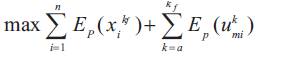
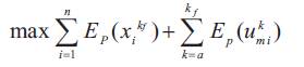
The main objective is to maximize the total potential energy of water stored in all the reservoirs. The formulation must take into account the fact that the water stored in one reservoir will be used in all its downstream reservoirs, hence, the water stored in the upstream reservoir is more valuable than that stored in the downstream reservoir [1].

 

Where,

k_f : Last period of the planning horizon.

Potential energy of water stored in reservoir i at the end of the planning horizon k_f. This energy depends on the amount of water x_i^kf stored in the reservoir i on its effective water head and on the effective water head of the downstream reservoirs.

Total potential energy of the released water u^k_mi from reservoir ,which will reach later the downstream reservoir i after the last period of the planning horizon k_f.

 

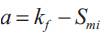
m : The reservoir immediately preceding the reservoir i.

S_mi : Time required for the water discharged from reservoir m to reach its direct downstream reservoir i in hours.

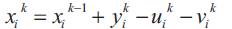
The principal operational constraints of the system are the following [1-2],[ 5-8]:- Hydraulic continuity constraint:

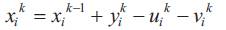
For each reservoir i at each time period k,the following constraint establishes the water balance equation:

 

Where,

x_i^k : Content of the reservoir i at period k in Mm³

u_i^k :Turbine discharge of hydroelectric plant i in period in k Mm^3.

v_i^k:Spillage of hydroelectric plant i in period k in Mm³.

y_i^k:Total inflows to reservoir i in period k in Mm³.

Taking into account hydraulic coupling, the total inflow to reservoirs is determined as follows:

 

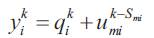
q_i^k :Natural inflows to reservoir i in period k in Mm³.

u_mi^k-Smi :Turbine discharge from hydroelectric plant m which will reach later the downstream reservoir i at period

 

Minimum and maximum storage limits

 

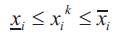
Lower and upper limits on reservoir storage capacity respectively, for reservoir i in Mm³.

Minimum and maximum discharge limits

 

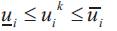
Minimum and maximum limits on water discharge, respectively, of hydroelectric plant.

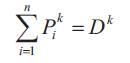
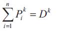
The total power generated by all the hydroelectric plants must satisfy the system load demand at each period of the planning horizon. In mathematical terms, this has the following form:

 

Where,

D^k:The demand for electrical power at each period k in Mw

P_i^k: Electric power generated by hydro plant k at period in Mw.

n:Number of reservoirs of the system

In mathematical terms, we formulate the short term scheduling problem of a hydroelectric plant system as follows [1]:

(1)

Subject to the following constraints

(2)

(3)

(4)

(5)

(6)

This problem can be solved by applying the discrete maximum principle as follows [1], 9-10]:

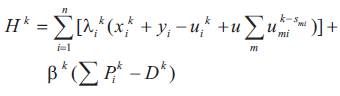
Associating the constraint (2) to the criterion (1) with the dual variable λ_i^k to satisfy the balance between electric energy demand and generation we associate the constraint (3) to the criterion (1) with the Lagrange multiplier β^kand then we define the function H^k called the Hamiltonian function, which has the following form:

(7)

The problem (1)-(6) becomes:

 

Subject to constraints (4)-(6), with the conversion equation of the associate variable [9]

(8)

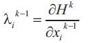
When constraints (4), (5) and (6) are inactive, the optimal trajectory  u_i^k will be reached when the following optimality conditions for each hydroelectric plant and at each period are satisfied.

(9)

In order to solve these equations, we need to know the boundary conditions, which are

(10)

(11)

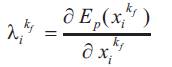
Consequently, equations (2) and (8)-(11) constitute a twopoint boundary value problem whose solution determines the optimal state and control variables. This problem is solved iteratively by using the gradient method.

To take into account possible violations of constraints (4) and (5) we proceed respectively as follows,

• The first one is the initial state, which is specified, i.e. at the initial time, the initial content of all reservoirs are known, thus
• The second one is the terminal condition for the ad joint equation
• If the value of sum u_i^k which satisfies the optimality condition (8) violates the constraint (5), we'll fix them to their boundary limits, the others are left free. Then a new research for the optimum is made but with only the free variables.
• To deal with possible violations of constraint (4), we use the augmented Lagrange method [1],[3],[11], which consists in adding a function R_i^k to the Hamiltonian H^k which penalizes the violation of constraints (5). Then the Hamiltonian H^k becomes

(12)

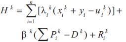
The function R_i^k is defined as follows

(13)

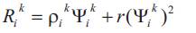
Where:

r :Penalty weight.

ρ_i^k : Lagrange multipliers, updated as follows

(14)

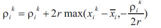
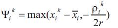
The function ψ_i^k is determined as follows:

(15)

In order to testify the efficiency and the performances of the method we apply the proposed algorithm to the system composed of four reservoirs in cascade located on the same river as shown in Figure 1 [4]. The characteristics of the system reservoirs and water time travel are shown in Table 1.

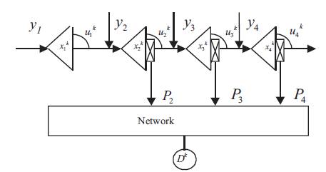
Figure 1. The Power System Configuration

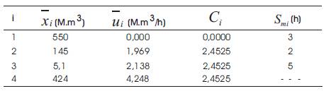
Table 1. Characteristics of The Installations

Where,

Maximal storage capacity of reservoir i

Maximal discharge capacity of reservoir

S_mi :Time taken by the water to travel from reservoir m to reservoir i

The following relation determines the water head [4]:

 

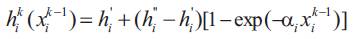
Where,

h_i^', h_i^'' , α_i , C_i Positive constants characterizing the reservoir.

The constant values of each reservoir are given in the following Table 2.

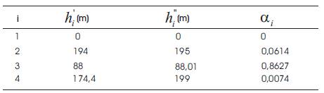
Table 2. Characteristics of Water Head

The natural flows q_i^k are assumed constant throughout the week at the four sites. Their values are given in Table 3 as well as the initial content x_i^o of each reservoir of the system:

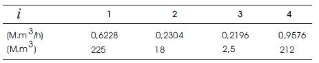
Table 3. Initial Contents and The Natural Inflows

The demand for electrical power Dk is shown in Figure 2.

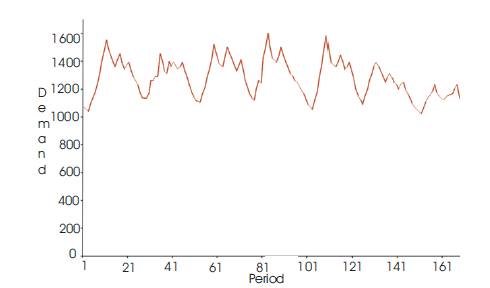
Figure 2. Weekly Demand For Energy

The optimal solution Figure 3 is obtained while satisfying all operating constraints after a very moderate number of iteration compared to that obtained by A. Turgeon [4] for the same system.

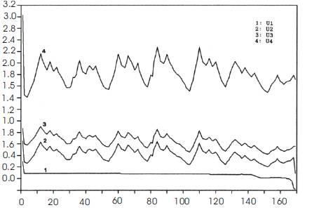
Figure 3. Optimal Discharge Trajectories

We can reduce this number by using an optimal step in the gradient method of our algorithm, and by adjusting adequately the penalty weight r factor. This will lead to a rapid exit from the violated zone as it is shown in Table 4. We state on one hand that the discharge follows the demand because the production is proportional to the discharge and must be equal to the demand. On the other hand, the discharge in the downstream reservoir is greater than the discharge in the upstream one, because the water stored in the upstream reservoir is more valuable than the water stored in the upstream one, i.e. the water of the upstream reservoir will also be used in the upstream ones. Consequently, in economic term water in the upstream reservoirs should be preserved as shown in Figure 3. Consequently, the reserve in potential energy of the system becomes more important, in spite of the considerable decrease in the contents of the downstream reservoirs. In addition, management is done without the draining of any reservoir as it is shown in Table 5.

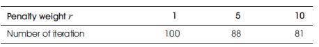
Table 4. Influence of penalty weight on iteration

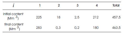
Table 5. Initial contents and final contents

The optimal management of hydroelectric system allows having the final contents of all the reservoirs higher than the initial contents as it is illustrated in Table 5.

The behavior of the objective function during the optimization process is illustrated in Figure 4. We note that the search for optimum is very slow when we approach the solution; this is due to the gradient method itself.

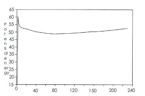
Figure 4. Behavior of the search trajectory (objective function)

With the discrete maximum principle, the optimal solution is obtained by solving simultaneous equations representing the optimality conditions, and it turned out to be efficient. And so was the augmented Lagrangian method. Hence the algorithm proposed requires moderate time and storage for its execution and can be applied efficiently to large dimensions problems

More improvements could be made to the proposed algorithm in order to increase the speed convergence of the algorithm and its execution time by improving the gradient method, and by adjusting adequately the penalty weight factor.

Taking into account the time delay between reservoirs increases considerably, the dimension of the problem.