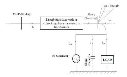
Figure 1. Basic Building Block of URDS inclusion of all Models
This paper presents a simple method of three phase power flow algorithm for application to unbalanced radial distribution systems (URDS) with inclusion of voltage regulators and transformer modeling. Distribution systems are usually unbalanced due to unbalanced loading at the different phases. In this paper forward - backward propagation algorithm is used to calculate branch currents and node voltages at each node. The proposed method has been tested to analyze several distribution networks. The application of this method is also extended to find optimum location for reactive power compensation and network reconfiguration for planning and day-to-day operation of distribution networks. The proposed method exactly finds out the critical lines as that of the conventional method. The effectiveness of the proposed method was successfully applied to 19 bus and 25 bus unbalanced radial test systems.
Load flow analysis is an important task for power system planning and operational studies. Certain applications, particularly in distribution automation and optimization of a power system, require repeated load flow solution and in these applications, it is very important to solve the load flow problem as efficiently as possible. As the power distribution networks become more and more complex, there is a higher demand for efficient and reliable system operation. Consequently, the most important system analysis tool, load flow studies, must have the capability to handle various system configurations with adequate accuracy and speed. In many cases, it is observed that the radial distribution systems are unbalanced because of single-phase, two-phase and three-phase loads. Thus, load flow solution for unbalanced case and, hence special treatment is required for solving such networks.
Due to the high R/X ratios and unbalanced operation in distribution systems, the Newton-Raphson and ordinary Fast Decoupled Load Flow method may provide inaccurate results and may not be converged. Therefore, conventional load flow methods cannot be directly applied to distribution systems. In many cases, the radial distribution systems include untransposed lines which are unbalanced because of single phase, two phase and three phase loads. Thus, load flow analysis of balanced radial distribution systems [1-3] will be inefficient to solve the unbalanced cases and the distribution systems need to be analyzed on a three phase basis instead of single phase basis.
There have been a lot of interests in the area of three phase distribution load flows. A fast decoupled power flow method has been proposed in [4]. This method orders the laterals instead of buses into layers, thus reducing the problem size to the number of laterals. Using of lateral variables instead of bus variables makes this method more efficient for a given system topology, but it may add some difficulties if the network topology is changed regularly, which is common in distribution systems because of switching operations. In [5], a method for solving unbalanced radial distribution systems based on the Newton-Raphson method has been proposed. Thukaram et al. [6] have proposed a method for solving three-phase radial distribution networks. This method uses the forward and backward propagation [7] to calculate branch currents and bus voltages. In recent years the three-phase current injection method (TCIM) has been proposed [8]. TCIM is based on the current injection equations written in rectangular coordinates and is a full Newton method. As such, it presents quadratic convergence properties and convergence is obtained for all but some extremely ill-conditioned cases. Further TCIM developments led to the representation of control devices [9], [10]. Miu et al., [11] have also proposed method for solving three-phase radial distribution networks. However, methods proposed by researchers reviewed above are very cumbersome and large computation time is required.
A fast decoupled G-matrix method for power flow, based on equivalent current injections, has been proposed in [12] .This method uses a constant Jacobian matrix which needs to be inverted only once. However, the Jacobian matrix is formed by omitting the reactance of the distribution lines with the assumption that R>>X; and it fails if X>R. In [14], a method has been suggested for three phase power flow analysis in distribution networks by combining the implicit Z-bus method [13] and the Gauss- Seidel method. This method uses fractional factorization of Y-bus matrix. Thus, large computational time is necessary for this method. The Network Topology method uses two matrices, viz. bus injection to branch current (BIBC) and branch-current to bus-voltage (BCBV) matrices, to find out the solution [15]. The Forward-Backward Substitution [15] and Ladder Network theory [16-18] based on approaches trace the network to and fro from its load end to source end.
Due to its low memory requirements, computation efficiency and robust convergence characteristic, Forward/Backward sweep-based methods have gained the most popularity for distribution load flow analysis in recent years. One of the distinguishing features of the radial distribution network is that there is a unique path from any given bus back to the source. This is the key feature exploited by the backward/forward sweep-based methods. There are several power flow methods based on backward/forward technique. They may be classified as,
The current summation method is used in this thesis as it is more convenient and faster than the power summation method because it uses only 'V' and 'I' instead of 'P' and 'Q'. Most of the methods are also proposed in the context of limited network modeling. In particular, none of the algorithms in the literature include modeling for transformers which are grounded on one side and ungrounded on the other. Unlike the extension from a single-phase to a three-phase representation, the addition of such modeling into the formulation is not straight forward. Line charging capacitance, cogeneration, and general load models are also typically not considered.
The purpose of this paper is to develop a new computation model for radial distribution network, which requires lesser computer memory and is computationally fast.
The proposed method is based on recursive algebraic equations.
This algorithm has been developed considering all types of loads. However, this algorithm can easily accommodate composite load modeling and it has good convergence property for practical unbalanced radial distribution networks.
In this paper, a simple method of load flow technique for unbalanced distribution systems is proposed. The proposed method involves only the evaluation of a simple algebraic expression of receiving end voltages. The mathematical formulation of the proposed load flow method is explained in the following section.
Radial distribution system can be modeled as a network of buses connected by distribution lines (with or without voltage regulators), switches or transformers. Each bus may also have a corresponding load, shunt capacitor connected to it. This model can be represented by a radial interconnection of copies of the basic building block shown in Figure 1. Since a given branch may be single-phase, two-phase, or three-phase, each of the labeled quantities is respectively a complex scalar, a 2 x 1, or a 3 x 1 complex vector.
Figure 1. Basic Building Block of URDS inclusion of all Models
For the analysis of power transmission line, two fundamental assumptions are made, namely,
However, distribution systems do not lend themselves to either of the two assumptions. Because of the dominance of single-phase loads, the assumption of balanced threephase currents is not applicable. Distribution lines are seldom transposed, nor can it be assumed that the conductor configuration is an equilateral triangle. When these two assumptions are invalid, it is necessary to introduce a more accurate method of calculating the line impedance.
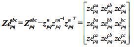
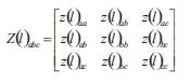
A general representation of a distribution system with N conductors can be formulated by resorting to the Carson's equations [18], leading to a N×N primitive impedance matrix. For most application, the primitive impedance matrices containing the self and mutual impedance of the each branch need to be reduced to the same dimension. A convenient representation can be formulated as a 3×3 matrix in the phase frame, consisting of the self and mutual equivalent impedances for the three phases. The standard method used to form this matrix is the Kron reduction, based on the Kirchoff's laws. For instance a four-wire grounded wye overhead distribution line shown in Figure 2 results in a 4×4 impedance matrix.
The corresponding equations are,
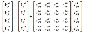
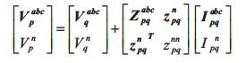
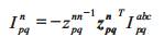
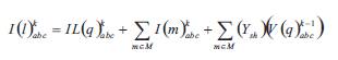
Ipqabc is the Current vector through line between bus p and q, can be equal to, the sum of the load currents of all the buses beyond line between bus p and q plus the sum of the charging currents of all the buses beyond line between bus p and q, of each phase.
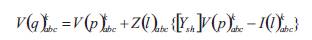
Therefore the bus q voltage can be computed when we know the bus p voltage, mathematically, by rewriting eqn.(4)
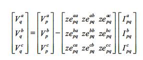
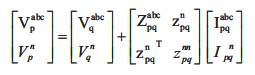
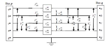
Figure 2. Model of the Three-phase Four-wire Distribution Line
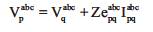
The previous line section model can be improved by the inclusion of line charging representation. The shunt capacitances phase to phase and phase to ground, depicted in Figure 3, can be taken into account through additional current injections.
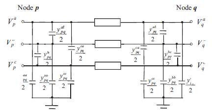
Figure 3. Shunt Admittance of Line Sections
In distribution systems loads can exist in one, two and three phase loads with wye or delta connections. Also loads can be categorized into three types depending on the load characteristics; constant power, constant impedance and constant current.
Mathematical models of these load types for both wye connected and delta connected are tabulated in Table1.
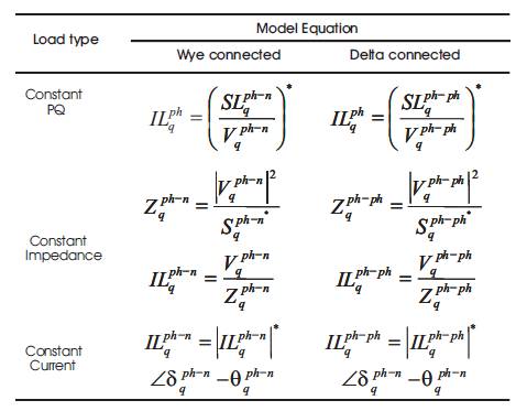
Table 1. Mathematical Models of Different Loads
Constant Power: Real and reactive power injections at the bus are kept constant. This load corresponds to the traditional PQ approximation in single-phase analysis.
Constant Impedance: These types of loads are useful to model large industrial loads. The impedance of the load is calculated by the specified real and reactive power at nominal voltage and is kept constant.
Constant Current: The magnitude of the load current is calculated by the specified real and reactive power at nominal voltage and is kept constant.
Sometimes the primary feeder supplies loads through distribution transformers tapped at various locations along line section. If every load point is modeled as a node then there are a large number of nodes in the system. So these loads are represented as lumped loads
The capacitor is modeled as a constant impedance matrix. The current injection into node k from a capacitor is
Switches are modeled as branches with zero impedance.
Forward sweep


The impact of the numerous transformers in a distribution system is significant. Transformers affect system loss, zero sequence current, grounding method, and protection strategy. Three-phase transformer is represented by two blocks shown in Figure 4, One block represents the per unit leakage admittance matrix YTabc and the other block models the core loss as a function of voltage on the secondary side.
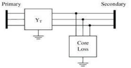
Figure 4. General Three-Phase Transformer Model
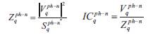
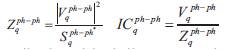
The core loss of a transformer [21] is approximated by shunt core loss functions on each phase of the secondary terminal of the transformer. Transformer core loss functions represented in per unit at the system power base are,
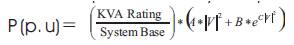
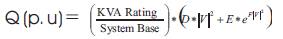
D=0.00167 E=0.268* 10-13 F=22.7
|V| is the voltage magnitude in per unit.
It must be noted that the coefficients; A, B, C, D, E, and F; are machine dependent constants. For the current project, core losses are represented by the functions and typical constants shown above.
For simplification, a single three-phase transformer is approximated by three identical single-phase transformers connected appropriately. This assumption is not essential; however, it simplifies the ensuing derivation and explanation. Based upon this assumption, the characteristic sub matrices used in forming the three phase transformer admittance matrices can be developed. Table 2 shows the sub-matrices of YT for the nine most common step-down transformer connection types, and Table 3 shows the matrices for step-up transformers.
Where
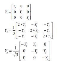
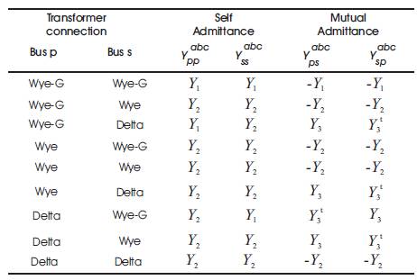
Table 2. YT Sub-Matrices for Common Step-Down Transformer Connections
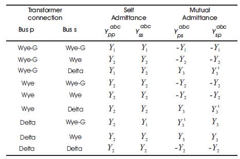
Table 3. YT Sub-Matrices for Common Step-Up Transformer Connections
If the transformer has an off-nominal tap ratio α:β between the primary and secondary windings, where are tappings on the primary and secondary sides, respectively, then the sub-matrices are modified as follows:
a) Divide the self admittance matrix of the primary by α2
b) Divide the self admittance matrix of the secondary by β2
c) Divide the mutual admittance matrices by αβ
With the nodal admittance matrix YTabc the transformer voltage-current relationship can be expressed as
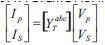
Where as
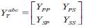
The matrix YTabc is divided into four 3x 3 sub matrices:Ypp , Yps , Ysp , Yss Vectors, Vp and Vs are the three- phase line-to-neutral bus voltages and Ip and Is injection currents at the primary and secondary sides of the transformer, respectively.
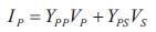
As described earlier, in backward sweep procedure,Vs and Is are known, while Vp and Ip are to be calculated. From (15), the following can be derived:

In forward sweep, Vp and Ip are known, and Vs needs to be calculated. Similarly
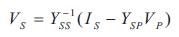
According to (16)–(18), the implementation of the forward/backward sweep algorithm requires the inversion of sub matrices Yss and Ysp. However, a close examination of the matrices for common transformer configurations shows that these sub matrices are often singular.
From the above tables Y1 , Y2 and Y3 it is observed that Ysp is invertible only for YG/YG connection, and is invertible only for and connections. For connection, (16)–(18) can be directly used for forward and backward sweep calculations. For ΔYG connection, only (18) can be used in forward sweep. For all other connection types, since the matrices are singular, there is no unique solution to the above equations. In essence, the singularity in those transformer configurations arises due to the lack of voltage reference point on one or both sides of the transformer.
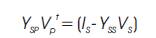
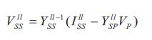
To circumvent the singularity issue, it is noted that although the three-phase line-to-neutral voltages Vp and Vs cannot be obtained by solving (16) and (18), the nonzerosequence components of the voltages can be uniquely determined. To illustrate this point [22] in the backward sweep, rewrite (16) as,
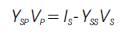
Let VpT represent the nonzero-sequence components of Vp
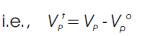
Where vector Vpo is the zero-sequence voltage on the primary side
Thus,
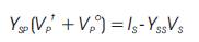
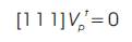
The product of Vsp and Vpois always zero for transformer configurations other than YG/YG . This is because Ysp is represented by Y2 or Y3 in all other transformer configurations except YG/YG . From Y2 and Y3 it can be seen that
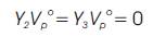
So (8) can be reduced to
Equation (10) indicates that the zero-sequence component of Vp
Does not affect the backward sweep calculation for transformers with a singular Ysp matrix. The above analysis show that (16) can be used to calculate both VP and its nonzero sequence components VPt and a modification is needed.
Equation (10) and(11) can be combined as
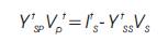
Where YtSPis obtained by replacing the last row of YSP with [ 1 1 1], while ItS and YtSS are same as IS and Yss except that elements in their last row are set to zero so that equation(24) is satisfied.
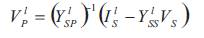
Now that Ytsp is not singular, the non zero sequence components of the voltages on the primary side can be determined by
Similar results can be obtained for forward sweep calculation.
Where Vllssis the nonzero sequence component of Vs ,Vllssobtained by setting the elements in the last row of ISYSP to 0, respectively.
Once the nonzero-sequence components of calculated, zero-sequence components are added to them to form the line-to-neutral voltages so that the forward/backward sweep procedure can continue.
A voltage regulator is a device that keeps a predetermined voltage in a distribution line in despite of the load variations within its rated power. It consists of an autotransformer able to increase or reduce its output voltage by means of automatic tap changing. The command of the commutation mechanism can be done automatically or by manual operation. A voltage regulator is equipped with controls and accessories for its tap to be adjusted automatically under load conditions. These accessories are sensitive to voltage variations as to keep the output voltage within a determined range. The most common device is a mono-phase regulator that can be used in mono-phase systems. For three-phase distribution systems, three mono-phase regulators can be connected in grounded wye or closed delta conforming a three-phase regulator bank. Alternatively, two regulators can be connected in open delta, in such a case, only two of the three voltages are controlled.
Voltage regulators can be connected in series throughout the feeder. The maximum number of voltage regulators connected in this way is limited by the electric losses or the thermal limit of the line. In long feeders two voltage regulators can be located, and in some cases up to three, being this, the maximum number recommended to be installed in a single feeder.
Type B regulator is used as the most common type of voltage regulator.
In type B regulator in the raise or lower position is the signal of the winding ratio (n1 /n2 ). The actual winding ratio in each winding is unknown, and the tap position is known. The equations of the effective winding ratio αR can be modified in function of the tap position. Each tap can change the voltage 5/8 % or 0.00625 in p.u, then the effective ratio is
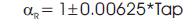
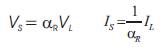
In (28) the negative signal refers to the raise position, and the positive refers to the lower position. The ratios of source voltage and current with respect to the load voltage and current are given by:
Type B:
Step1. Read the given data of regulator
Step2. Read the branch current in which regulator is inserted from the backward sweep
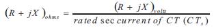
Step3. Find the CT ratio for three phases as

Where as CTs = 5 Amps,
Step4.Convert the R and X values from volts to ohms as
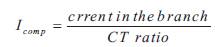
Step5. Calculating current in the compensator
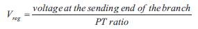
Step6. Calculate the Input voltage to the compensator as
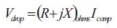
Step7.Voltage drop in the compensator circuit is
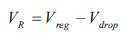
Step8. Voltage across the voltage relays in three phases
Step9. Finding the tapping of the regulator
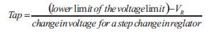
Step10. Voltage output of the regulator
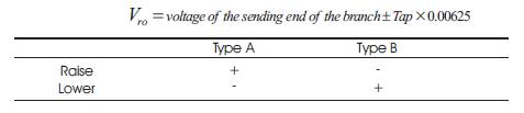
‘+’ For raise
‘-’ For lower
Step11. End
For the three phase network generally three single phase regulators are connected in desired configuration.
The purpose of the backward sweep is to update branch currents in each section, by considering the previous iteration voltages at each node. During backward propagation, voltage values are held constant at the values obtained in the forward path and updated branch currents are transmitted backward along the feeder using backward path. Backward sweep starts from extreme end branch and proceed along the forward path. Figure 5 shows phase a of a three-phase system where lines between nodes p and q feed the node q and all the other lines connecting node q draw current from line between node p and q. Figure 6 show the simple part of distribution network.
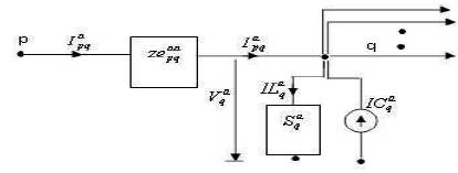
Figure 5. Single Phase Line Section with Load Connected at Node q between to Phase 'a' and Neutral n.
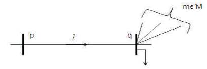
Figure 6. Simple Part of Distribution Network
During this propagation load currents, capacitor currents (if exist) using equations in Table 1 and equations 8 and 9 are calculated respectively. The half line charging shunt currents of all the branches at the node are added to the load current. Once the child node current is calculated, the parent branch current can be calculated using eqn. (30).
Where Ysh is the half line shunt admittance of the branch,I(i)kabc is the branch current vector in line section l, and I(m)kabc is the current vector in branch m before updating, M represents the set of line sections connected to lth branch and k is the iteration.
If capacitor bank is placed at the receiving end of the branch then capacitor current should also be included.
The purpose of the forward sweep is to calculate the voltages at each node starting from the source node. The source node voltage is set as 1.0 per unit and other node voltages are calculated using the eqn. (31).
Where , V(p)kabc,V(q)kabc are the voltage vectors of phases for pth and qth buses respectively.
These calculations will be carried out till the voltage at each bus is within the specified limits. At this point the voltages at each node, and the currents flowing in all line segments are known, which are used to find the power losses in each line segment. Therefore the real and reactive power losses in the line between buses p and q may be written as,
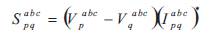
Where Spqabc is a vector of power loss with three, two or single phase, Vpabcand Vqabc are voltage vector of three phases at buses p and q respectively and Ipqabc is the branch current vector of three phases for the section connected in between pth and qth buses.
Step1. Read input data regarding the unbalanced radial distribution system.
Step2. Initialize the voltage magnitude at all buses as 1p.u and voltage angles to be 00 , -1200 , 1200 for phase-a, phase-b and phase-c respectively.
Step3. Set iteration count k=1 and ∈= 0.0001
Step4. Calculate effective current injection at all buses, which is the sum of load current, line charging current, capacitor current and co-generator currents.
Step5. A backward sweep is started from the leaf buses to calculate the branch currents.
This can be done in two steps as follows,
I. Finding the effective current at each bus
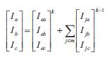
Ika= current in the phase-a, at kth level bus.
Ieak= effective current injected in phase-a, at level bus, calculated in step 4.
Ijak-1= effective current at the jth adjacent bus in the (k-1)th level.
Similarly for phase-b and phase-c.
I. Assigning the effective bus currents to the branches as

Ipqabc - Branch current, connected between buses p and q and
Iqabc - Effective current at bus q.
Step 6. A forward sweep is started to update bus voltage magnitudes starting from the source bus towards end buses using equation (6).
Step 7. Convergence is checked for each of the bus voltage magnitude comparing with the previous iteration. If the difference is less than ∈ step 8 is followed else set k=k+1 and go to step 4.
Step8. Calculate the real and reactive power losses at each bus.
Step9. Print voltages and power losses at each bus and stop.
Computer program for radial distribution load flow has been developed incorporating the above power algorithm. This program was developed in MATLAB 7.0. This program computes the power flow solution for its given radial network with its loadings. The performance of the system is evaluated on two examples of unbalanced radial distribution system to find voltage profile, branch loading and power losses.
The 11 kV, 19-bus unbalanced radial distribution system [19] is shown in Figure 7. The line, load and tie switch data are given in Appendix A1. For the load flow, base voltage and base MVA are chosen as 11 kV and 1000 KVA respectively. The results of voltage profile by load flow program are shown in Table 5. Table 6 shows the power flows in the phases of each branch of 19 bus URDS. The convergence solution is obtained in 4 iterations and time taken is 0.00659seconds. The total real and reactive power losses are 13.4729 kW and 5.7965 kVAR respectively.
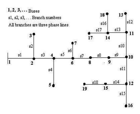
Figure 7. Single Line Diagram for 19 Bus URDS
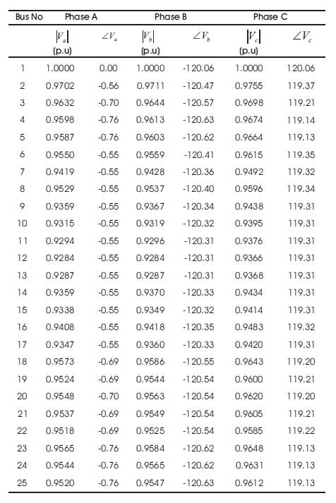
Table 4. Voltage Profile for the 25–Bus URDS
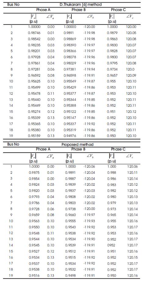
Table 5. Voltage Profile for the 19–Bus URDS
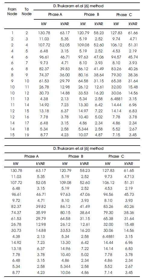
Table 6. Power Flows in the Phases of each Branch of 19-Bus URDS
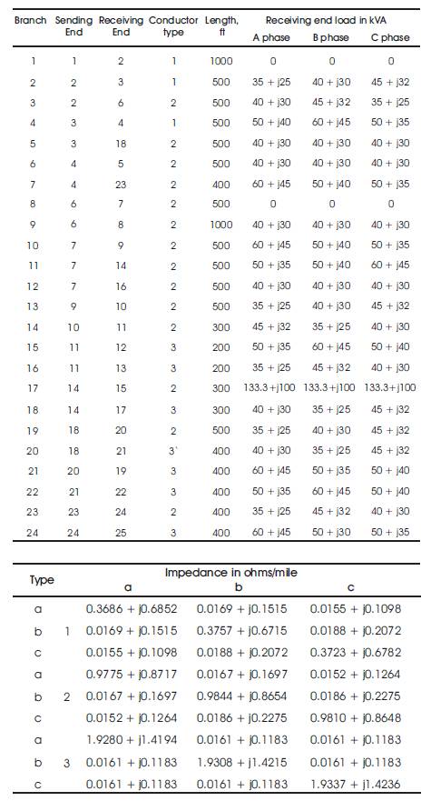
The proposed algorithm is tested on IEEE 25-bus unbalanced radial distribution system [19] as shown in Figure 8. The line and load data are given in Appendix A2. For the load flow, base voltage and base MVA are chosen as 4.16 kV and 30 MVA respectively. The results of voltage profile by load flow program are shown in Table 4. Table 7 shows the power flows in the phases of each branch of 25 bus URDS. The convergence solution is obtained in 5 iterations and time taken is 0.12364 seconds. The total real and reactive power losses are 150.1225 kW and 167.3086 kVAR respectively.
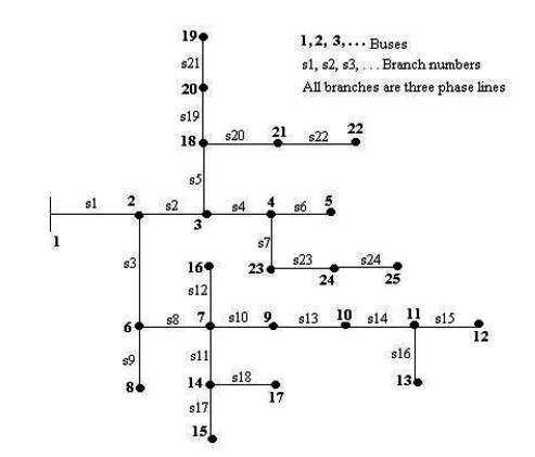
Figure 8. Single Line Diagram of 25-Bus URDS
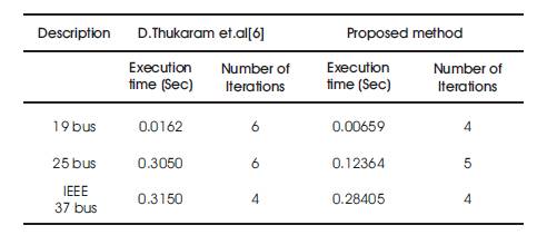
Table 7. Summary of Test Results
The results obtained by proposed method are compared with those given in [6] which are shown in Table 8. The effectiveness of the proposed method is compared in terms of number of number of iterations and CPU time. The number of iterations, and CPU time were lesser for the proposed method when compared with that of the Thukaram et. al method. Hence the proposed method is observed as the superior method when compared with method in [6].
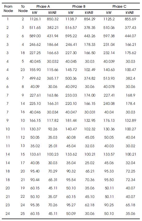
Table 8. Power Flows in the Phases of the Branch of 25 Bus URDS
In this paper, a simple and efficient computer algorithm has been presented to solve unbalanced radial distribution networks. In this paper a three phase load flow solution is proposed considering voltage regulator and transformer with detailed load modeling. The proposed method has good convergence property for any practical distribution networks with practical R/X ratio. Computationally, this method is extremely efficient, as it solves simple algebraic recursive equations for voltage phasors. Another advantage of the proposed method is all the data is stored in vector form, thus saving enormous amount of computer memory. The proposed method finds extensive use in network reconfiguration, capacitor placement and voltage regulator placement studies.
Table A1 Load data and line connectivity of 19-bus unbalanced system
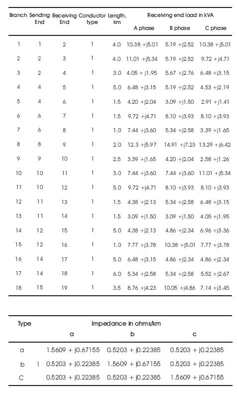
Table A2 Load data and line connectivity of 25-bus unbalanced system