Convolution

Convolution is a mathematical operation that gives the information about how the shape of one function is modified by other. It is defined as an integral of one function with the reverse and shifted form of other.

Convolution techniques of a discrete time signal are classified as two types as follows,

• Linear Convolution
• Circular Convolution

Linear Convolution

Linear convolution which is a fundamental computation in Linear time-invariant (LTI) systems, which is implemented using Verilog HDL. Simulation and synthesis are verified in Xilinx 10.1 ISE. Linear and time-invariant systems are an important class of systems and have significant signal processing applications. A Linear time invariant (LTI) system is completely characterized by its impulse. The impulse response is the response of a system to impulse signal or sequence.

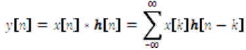
In discrete time, the output of linear convolution is the product of reverse and shifted version of the input sequence with impulse response of the system (Bharathi, Rani, &Varadrajan, 2013). It is given as,

(1)

h[n] is the system when input signal is applied as impulse sequence, δ[n]. To execute discrete time convolution, the input sequence and system response are duplicated together for -∞ < k < ∞ and the items are summed to compute yield tests of y[n]. Convolution entirety serves as an unequivocal realization of a discrete-time direct framework (Oppenheim & Schafer, 1975).

Practically, it is difficult to store a long duration input sequence. Therefore, in order to perform linear convolution of such a long duration input sequence with the impulse response of a system, the input sequence is divided into blocks. The successive blocks are processed one at a time and the results are combined to obtain the output sequence. The blocks are filtered separately and results are combined using overlap save method or overlap adds method.

Overlap-Save Method

Let the length of long duration input sequence be L. The length of impulse response = M. The input sequence is divided into blocks of data. The length of each block is N= L+M-1. Each block consists of last (M-1) data points of previous block followed by L new data points for first block of data. The first M-1 points are set to zero.

Therefore blocks of input sequence are

x1(k)= {0,0….0, x(0), x(n)…. x(L-1)}The first (M-1) samples are zeros.

x2(k)= {x(L-M+1)… x(L-1), x(L)… x(2L-1)}x(L-M+1)… x(L-1) are the last (M-1) samples

x3(k)= {x(2L-M+1)… x(2L-1), x(2L)… x(3L-1)}x(2L-M+1)… x(2L-1) are the last (M-1) samples from x2(k) x(2L)…. x(3L-1) are the L new samples

The length of impulse response has increased by appending L-1 zeros.

Overlap-Add Method

In this method, also the long direction input sequence is divided into blocks of data.

The length of each block is N= L+M-1.

The data blocks are represented as,

x1(k)= {x(0), x(1)… x(L-1), 0,0…}

x2(k)= {x(L), x(L+1)… x(2L-1), 0,0…}

x3(n)= {x(2L), x(2L+1)… x(3L-1), 0,0…}

Similarly, the length of impulse response has increased to L+M-1 by appending L-1 zeros to it. Circular convolution is performed on each block of input sequence with the impulse response to have blocks of output sequences. The last M-1 samples of each block of output sequence is overlapped and added to the first M-1 samples of succeeding block. The samples thus obtained are arranged in sequential order to have the final output sequence y(n). So, this method is called as Overlap-Add method.

Circular Convolution

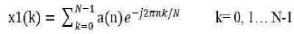
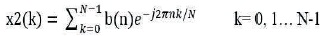
Let x1(k) and x2(k) be two finite- duration sequences of length N(Bharathi & Rani, 2003). Their respective N-point DFT's are

(2)

(3)

If two DFT's are multiplied together, the result is the sequence x3(k) of length N.

The relationship between X3(K) and sequences X1(k) and X2(k) is

(4)

(5)

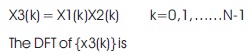
The multiplication of the DFT's of two sequences is equivalent to circular convolution of two sequences in the time domain. The methods that are used to find the circular convolution of two sequences are Concentric circle method and Matrix multiplication method.

Concentric Circle Method

The length of x1(k) should be equal to length of x2(k) in order to perform circular convolution using concentric circle method.

The three cases includes,

The length L of sequence x1(k) is equal to length M of sequence x2(k), direct procedure has to be applied.

If L>M, then M is made equal to L by adding L-M number of zero samples to the sequence, x2(k)

If M>L, then L is made equal to M by adding M-L number of zero samples to the sequence x1(k)

Matrix Multiplication Method

Circular convolution of two sequences x1(k) and x2(k) is obtained by representing the sequences in matrix form as shown in equation (6).

(6)

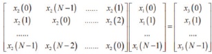
The columns of NxN matrix is formed by repeating the samples of x2(k) via circular shift. The elements of column matrix are the samples of sequence x1(k). The circular convolution of two sequences, x3(k), is obtained by multiplying NxN matrix of samples of x2(k) and column matrix, which consists of samples of x1(k).

1.1 Linear to Circular Convolution

Algorithm: Let x(n) be the input arrangement and h(n) be the impulse response of a directly time invariant system.

x(n)={x1,x2,x3} h(n)={h1,h2,h3}

• Find the maximum number of test display within the x(n) and h(n). K=max {no of tests of x(n), no of tests of h(n)}=Max(5,3)=5.
• Now discover the direct convolution of x(n) and h(n). Output of straight convolution is y_L (n)= {l₇, l₆, l₅, l₄, l₃, l₂, l₁, l₀}
• Consider k tests from l_n to l_n-k and include them with the n remaining tests display in yield of straight convolution.

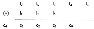
Y_c(n)= {c₄, c₃, c₂, c₁, c₀} is the output of circular convolution.

Example:

x(n)={1,2,3,4,5} h(n)={1,1,1}

Step 1: Maximum number of samples is k=5,

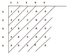
Step 2: Output of linear convolution is,

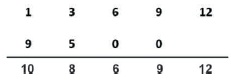
Y(n)= {1, 3, 6, 9, 12, 9, 5, 0, 0}

Step 3: The output of circular convolution is,

y(n)= {10, 8, 6, 9, 12}

1.2 Modified Booth Multiplier

Booth increases the calculation that comprises of three major steps as appeared in structure of Booth calculation figure that incorporates era of halfway item called as recoding, decreasing the halfway item in two lines, and expansion that gives last item (Wang, Kuang, & Liang, 2009). It is conceivable to diminish the number of halfway items by half, by utilizing the method of radix-4 Booth recoding. The fundamental idea is that, rather than moving and including for each column of multiplier term and increasing by 1 or 0, each moment column is taken and duplicated by ± 1, ± 2 or 0, to get the same results. In Radix-4 Booth encoder performs the method of encoding the multiplicand based on multiplier bits (Muralidharan & Chang, 2013). It'll compare 3 bits at a time with covering strategy. Gathering begins from the LSB, and the primary piece as it employs two bits of the multiplier and accept a zero for the third bit.

Radix-4 Booth calculation is given by Panyam and Bharathi (2012).

• Amplify the sign bit 1 position in case vital to guarantee that n is indeed.
• Add ‘a’ to the LSB of the multiplier.
• Agreeing to the esteem of each vector, each halfway item will 0,+y, y,+2y, -2y (Rabaey, Chandrakasan, & Nikolić, 2003).

Modified Booth multiplier Radix -4 recoding is shown in Table 1.

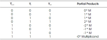
Table 1. Existing Modified Booth Recoding

Here, M=Multiplicand

Table 2 shows the comparison between different convolution techniques using modified booth multiplication.

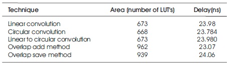
Table 2. Comparison between Different Convolution Techniques using Modified Booth Multiplication

2.1 Linear Convolution

Figure 1 shows the simulation results of linear convolution.

Consider input sequence as x(n)= {x3,x2,x1,x0}

Impulse sequence as h(n)= {h3,h2,h1,h0}

In both sequences all the values are of length4 bits

The given inputs are x(n)= [ 4, 3, 2, 1 ]

Impulse sequence is h(n)= [1, 1, 1, 1 ]

Output in decimal format is (Each of 8 bit length)

Y(n)= [4,7,9,10,6,31]

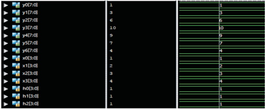
Figure 1. Simulation Results of Linear Convolution

2.2 Circular Convolution

Figure 2 shows the simulation results of circular convolution.

consider input sequence as a(n)= [a3,a2,a1,a0]

Impulse sequence as b(n)= [b3,b2,b1,b0]

In both sequences all the values are of length 4 bits

Input sequence is given as a[n]= [4,3,2,1]

Impulse sequence is given as b(n)= [3, 3, 2, 1 ]

Output in decimal format is (Each of 8 bit length)

Y(n)= [19,22,25,24]

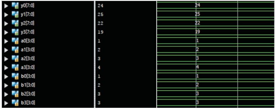
Figure 2. Simulation Results of Circular Convolution

2.3 Linear to Circular Convolution

Figure 3 shows the simulation results of linear to circular convolution.

Here input sequence is a(n)= [a3,a2,a1,a0]

Impulse sequence is b(n)= [b3,b2,b1,b0]

In both sequences all the values are length of 4 bits

The given inputs are a(n)= [ 4, 3, 2, 1]

Impulse sequence is b(n)= [3, 3, 2, 1]

Output in decimal format is (Each of 8 bit length) Y(n)= [19,22,26,24]

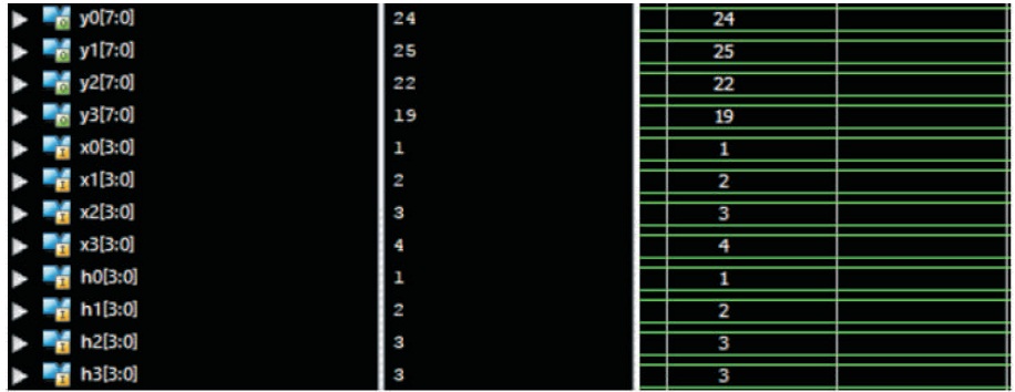
Figure 3. Simulation Results of Linear to Circular Convolution

2.4 Linear Convolution for Long Sequences

Figure 4 shows the simulation results of linear convolution using overlap add method.

2.4.1 Overlap Add Method

consider input sequence as i(n)= [i7,i6,i5,i4,i3,i2,i1,i0]

Impulse sequence is h(n)= [h3,h2,h1,h0]

In both sequences all the values are length of 4 bits

The given inputs are x(n)= [ 7, 6, 5, 5, 4, 3, 2, 1 ]

Impulse sequence is h(n)= [ 1, 1, 1 ]

Output in decimal format is (Each of 8 bit length)

g(n)= [7,13,18,16,14,12,9,6,3,1 ]

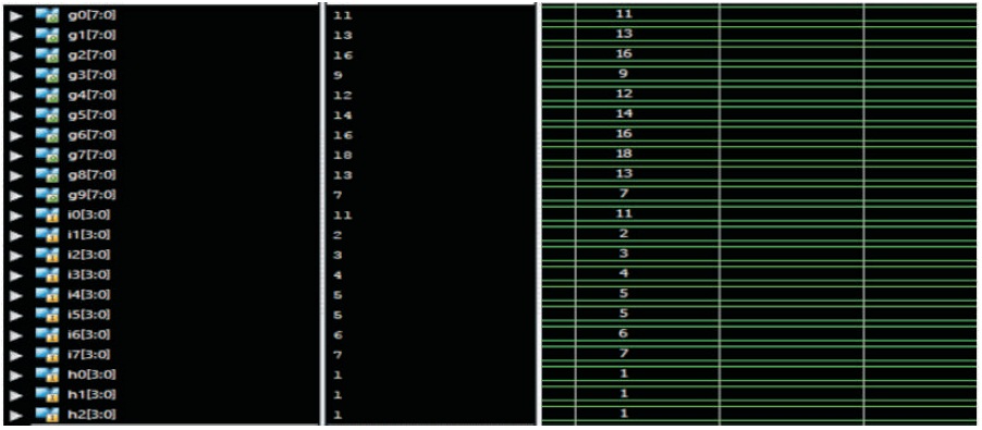
Figure 4. Simulation results of Linear Convolution using Overlap Add Method

2.4.2 Overlap Save Method

Figure 5 shows the simulation results of linear convolution using overlap save method.

consider input sequence as i(n)= [i7,i6,i5,i4,i3,i2,i1,i0]

Impulse sequence is h(n)= [h3,h2,h1,h0]

In both sequences all the values are length of 4 bits

The given inputs are x(n)= [ 7, 6, 5, 5, 4, 3, 2, 1 ]

Impulse sequence is h(n)= [ 1, 1, 1 ]

Output in decimal format is (Each of 8 bit length)

g(n)= [7,13,18,16,14,12,9,6,3,1 ]

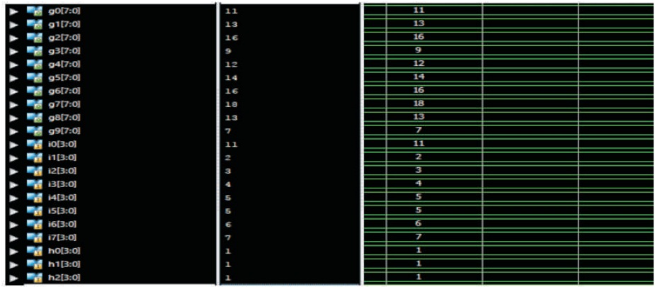
Figure 5. Simulation Results of Linear Convolution using Overlap Save Method

The main aim of this paper is to present a strategy for calculating the circular convolution by utilizing linear convolution. The execution time of the proposed strategy for convolution utilizing altered booth duplication calculation is compared with that other convolution techniques. By this strategy the circular convolution of long groupings utilizing direct convolution has obtained. To precisely analyze proposed framework, plan is coded utilizing the Verilog HDL dialect and synthesized it for FPGA items utilizing ISE. The proposed circuit takes approximately 23.98 ns to total 90 nm handle innovation gadgets. Additionally, the displayed concept can be expanded on an NXN case. Key component behind this is to maintain a strategic distance from the matric increase to urge circular convolution.