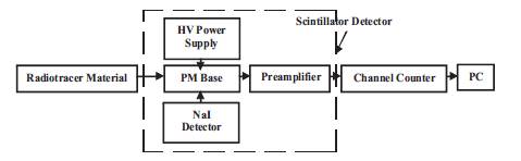
Figure 1. Block Diagram for RTD Signal measurements
This paper discusses the signal preprocessing of the acquired radiation signal for Residence Time Distribution (RTD). Radiation signals of Molybdenum-99 (Mo99 ) were acquired through system setup. This system begins with a scintillator detector, channel counter and a Personal Computer (PC). Different forms of noise are accompanied with the RTD radiation signal. Consequently, an algorithm was proposed based on signal processing. This algorithm depends on background correction, base line restoration, statistical error computation, radioactive decay correction and dead time correction methods. Therefore, background correction was performed using two independent methods. These methods are the minimum value of the RTD radiation signal method and the subtraction method. Then, base line restoration was performed. Statistical error of the RTD radiation signal was computed. However, two different methods were studied for radioactive decay correction. Moreover, a dead time correction method is proposed. Therefore, dead time percent is obtained. Consequently, the number of lost pulses is investigated. The accuracy of the considered algorithm is determined based on statistical measurements of the acquired RTD signal. A remarkable accuracy of the dead time measurements is observed.
The investigation of flow patterns and mixing in a fluid system is a well established field of chemical engineering. This field was developed to enable engineers to understand the flow behaviour of a chemical reactor, without having to account for the complete history of each fluid element. In his pioneering paper, Danckwerts (1953) pointed out that in place of such a complete description of the flow pattern, it is enough to know how long the fluid elements stay in the reactor. This is, of course, the Residence Time Distribution of the system [1]. Residence Time Distribution (RTD) has become an important tool for the analysis of industrial units and reactors. The RTD of fluid flow in process equipment determines their performance. Radiotracers are the methods of choice for obtaining the RTD in industrial processing vessels and wastewater treatment systems. Radiotracer RTD method has been extensively used in industry to optimize processes, solve problems, improve product quality, save energy and reduce pollution [2] . The Residence Time Distribution (RTD) and the actual mean residence time estimations from theoretical relationships are complex due to the presence of three components (solid mineral, balls and water), mass transport characteristics and segregation affecting solid holdup. Therefore, the experimental RTD determination is suitable for the industrial applications. The RTD was measured using the radioactive tracer technique. This technique allows for non-invasive tracer detection in order to characterize the solid and liquid mixing regimes without disturbances [3]. An analysis of the experimental RTD data provides valuable information about the fluid flow behavior, the degree of radial and axial dispersion, and possible flow problems in the exchanger, such as stagnation or short-circuiting. It is therefore important to perform a RTD study, complemented with temperature profile measurements, in order to assess the influence of the operating conditions on the fluid flow behavior and on the efficiency of the thermal treatment applied to the product, so as to optimize the crystallization process [4]. The topic of RTD has a lot of attention in the research. It is important for multiple industrial applications.
Therefore, a short survey was prepared that related to this topic. Kasban et al., 2010 [5] present three laboratory experiments that have been carried out using the Molybdenum-99 (Mo99 ) radiotracer to measure the Residence Time Distribution (RTD), the mixing time and the flow rate in a water flow rig. Their results show that the mixing time is inversely proportional to the rotation speed. Also, H. Kasban et al., 2010 [6] discussed some industrial radioisotope applications. They concluded that radioisotopes can be used to troubleshoot and optimise several industrial processes.
H. Kasban et al., 2011 [7] present a proposed method for RTD signal identification based on Power Density Spectrum (PDS). The cepstral features are extracted from the signal and from its linear and nonlinear modified periodograms. An Artificial Neural Network (ANN) is employed for training and testing the proposed method. O. Zahran et al., 2012 [8] reported that, RTD can be used for optimizing the design of industrial systems and determining their malfunctions. H. Kasban and Ashraf Hamid 2014 [9] presents an improvement for the RTD signal recognition method that is based on Power Density Spectrum (PDS). The features are extracted from the signals and from their Higher Orders Statistics (HOS) (Bispectrum and Trispectrum) instead of PDS. Seungkwon Shin et al., 2003 [10] presented a Residence Time Distribution (RTD) measurement method using a radioisotope tracer. They investigated a mathematical RTD model to represent the flow behavior and the existence of stagnant regions in the reactor. The objective of this work is to study different algorithms for RTD signal treatments. Therefore, this paper is organized as follows: in section 1, we present the experimental setup. Proposed algorithms are considered in section 2. Results and deeply discussion are summarized in section 3. The final section is devoted to a conclusion.
In this system, the components of the system for signal processing algorithms are described. It contains the following elements; Molybdenum-99 (Mo99 ) radiation point sources, scintillator detector with NaI(TI), channel counter and personal computer. Figure 1 depicts a block diagram of the considered system for RTD measurements. Scintillation detector with NaI(TI) is used to detect the radiation signal from Mo99 radiation sources. Consequently, an algorithm describing the dead time correction of RTD measured signal is introduced in Figure 2.
Figure 1. Block Diagram for RTD Signal measurements
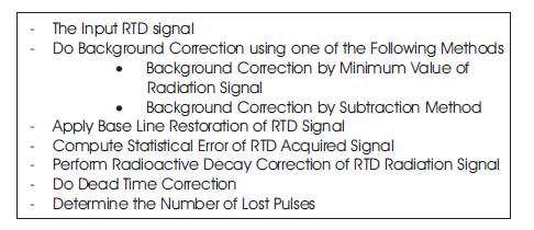
Figure 2. Dead Time Correction Algorithm of acquired RTD Radiation Signal
The detected gamma rays come not only from the source, one trying to measure, but also from other sources [11]. Radiation not originating from the ground is regarded as background [12]. The background corrections are the largest and most difficult correction to make.
There are two significant sources for background radiation. These are cosmic rays and radon decay products [13]. Cosmic rays are fast-moving particles from the space that enter the Earth's atmosphere along with their decay products. Since, the atmosphere absorbs some of these particles, the rate of detection of cosmic rays increases with increasing altitude. It is essential to take into account this background gamma at low activity measurements. Therefore, two different methods are applied on the acquired RTD signal.
Here, we are interested in removing the existing background radiation by applying the following formula [14],
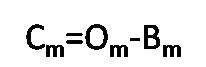
where Cm , Om , and Bm denote the background corrected signal, original signal, and minimum value of the original signal, respectively.
The Molybdenum-99 (Mo99 ) radiation signal was measured. Then, the radiation source is moved away from the radiation detector and the detector is exposed to the free air. Subsequently, subtract the acquired background signal from the measured one according to the following relation:
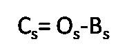
where Cs, Os and Bs denote the background corrected signal, acquired 60Co radiation signal, and background signal, respectively.
The corrected background RTD signal is shifted to be below the base line. However, it is important to restore the corrected signal to be above the x-axis line or the base line of RTD signal. This is done using the following formula.
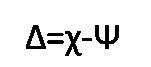
where Χ and Ψ denote the background corrected signal and minimum count in the background corrected signal, respectively.
Radioactive decay is a process, subject to inherent random variation [15]. It is randomly occurring events. Therefore, it must be described quantitatively in statistical terms [16]. There is a fluctuation in the decay rate of a particular sample from one instant to the next due to the random nature of radioactive decay and the half-life of the radionuclide. The theoretical standard deviation of counts can be calculated from the following formula.
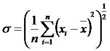
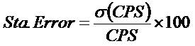
where  is the mean of the dataset x and n denotes the vector length of the datasets x. The previous equation can be rewritten by [15],
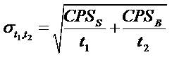
where CPSs and CPSB denote signal CPS at time t1 and background CPS at time t2 , respectively. Also, the time of measurements t1 is equal to t2 . Therefore, the standard error is given by [15],
Radioactive decay occurs with the emission of particles. Also, it may occur with an electromagnetic radiation from an atom due to a change within its nucleus [17]. The activity of any radionuclide decreases at a known rate. The value of the decay half-life is an important parameter. It appears inside an exponential function [18]. Therefore, its uncertainty must be carefully evaluated. Since, it may distort the results of the whole analysis. There are two different methods used to correct the radioactive decay. Those are depending on two different formulas. It is impossible to predict the exact moment at which a particular atom will decay. Each radioisotope has a characteristic rate of disintegration. It is proportional to the number of nuclei present. Thus, the rate of change of number of nuclei presents [19],
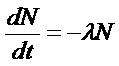
where N, dN and dt denote number of nuclei present at that time, the number of nuclei and decay short time, respectively. This equation is solved and given by [19]
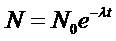
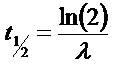
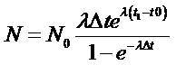
where N0 and are the number of radionuclide present at time (t=0), and the decay constant, respectively. If, N=N0/2, it yields
The activity of the source is measured. This activity decreases exponentially over time with the same half-life. However, one must measure the activity in a certain period of time in order to calculate the Counts Per Second (CPS) value. The result is imprecise as the sample decays during the measurement period. This does not usually occur. However, this phenomenon becomes noticeable in specific isotopes. Consequently, another precise formula was used for the computation of radioactive decay [15]. It is stated as,
where t1 , t0 and Δt denote the time when measurement started, reference time, and the measurement time, respectively.
All detector systems have a minimum amount of time that must separate two gamma photons in order that they are recorded as two separate pulses. This minimum time delay (or dead time, τ) may be due to either the physical detection process itself or the associated electronic devices [2]. High counting rate causes a high fractional dead time during measurements. Therefore, it decreases rapidly during the measuring time. Several authors proposed corrections by means of additional electronic circuits. However, other investigated different mathematical solutions for dead time correction [20- 21]. Consequently, the true count rate is given by,
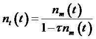
where τ and nm (t) denote dead time and the measured count rate, respectively. Thus, the true rates were computed depending on equation (10). These calculations are based on signal processing process.
Two different methods are used for background correction of the acquired RTD radiation signal. These methods are the minimum value of the radiation signal method and the subtraction method. The result of the first method is shown in Figure 3 (a). The obtained result confirms that 115 counts per seconds of minimum value of the original RTD signal were discovered.
The result of the second method is depicted in Figure 3(b). However, we concluded that the background subtraction method introduces better results. Therefore, it is more accurate than the minimum value method. Consequently, it represents the actual background signal. Since, the background is varied at every instance and not static. Therefore, the proposed work continues using the subtraction method. Moreover, a quantitative evaluation of the considered background correction methods are depicted in Table 1. The obtained results confirm the superiority of background subtraction method over minimum value of the RTD signal method. However, the obtained RTD signal lies below the base line. Consequently, other preprocessing step is necessary.
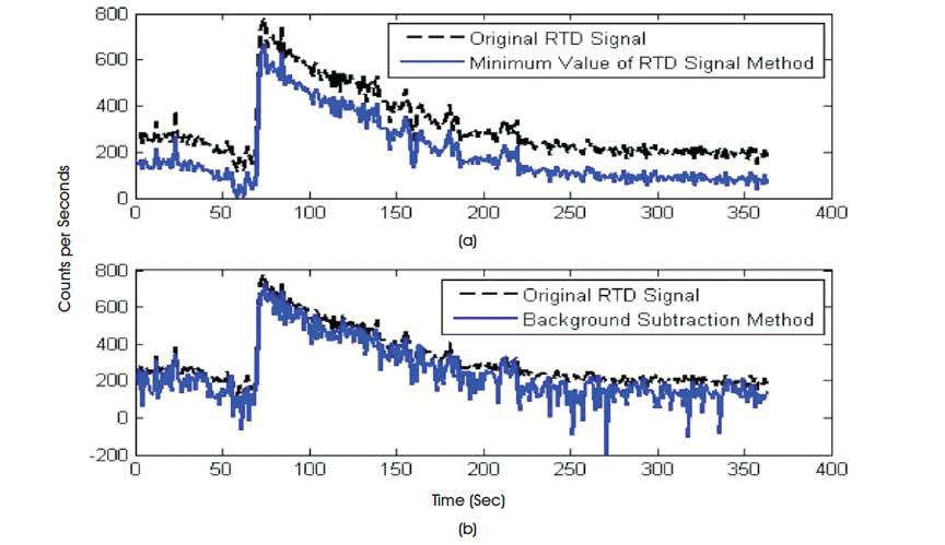
Figure 3. Background corrected methods using Minimum value of the RTD signal method Background Subtraction Method
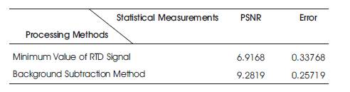
Table 1. Quantitative evaluation of Background Correction Methods
The output of previous step is the input of current one. Therefore, the base line restoration method was applied for restoration of the RTD signal. This method was applied for the background subtraction method only, as illustrated in Figure 4. The evaluation of this method is illustrated through statistical measurements in Table 2. Although, the minimum value of RTD signal shows less efficient results. It does not need the base line restoration.
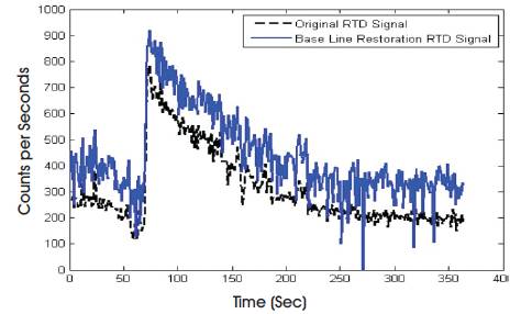
Figure 4. Base Line Restoration of the Background Correction RTD signal by Subtraction Method
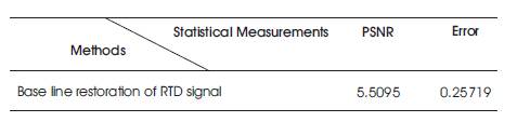
Table 2. Statistical evaluation of Base Line Restoration method of RTD Signal
It is essential to compute the statistical errors of the acquired RTD signal. These computations are based on analytical methodology. Therefore, the standard deviation and statistical error were computed as depicted in Table 3.
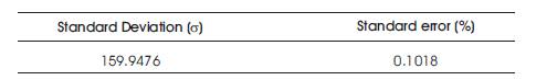
Table 3. Statistical Parameters of acquired RTD Radiation Signal
There are two different analytical methods used for the correction of radioactive decay. These methods are depending on two different methods. The result of the first method is shown in Figure 5 (a). However, the result of the second method is depicted in Figure 5 (b). Also, comparison between these two methods are conducted as depicted in Table 4. The obtained result confirms that the first analytical method introduces efficient results.
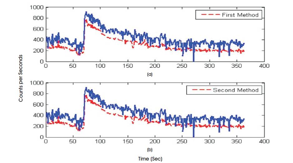
Figure 5. Decay correction methods using a) 1st Analytical method b) 2nd Analytical method
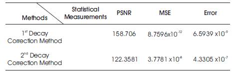
Table 4. Quantitative evaluation of Decay Correction Methods for RTD Radiation Signal
The efficient methodology for dead time is presented for correct RTD signal measurements. Therefore, the dead time of the experimental measurement was computed. It depends on system components and detection system [22]. The calculation in Table 5 shows a dead time of 15.783μs and number of recovered pulses is 3.0126x10⁴ counts.
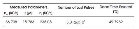
Table 5. Dead Time Correction Results of99 Mo RTD measured Signal
Residence Time Distribution is an important topic for industrial applications. Consequently, system configuration for signal acquisition is conducted. Therefore, an algorithm for signal reprocessing is considered. This algorithm is based on background correction, base line restoration, statistical error calculation, radioactive decay correction and dead time correction algorithms. Thus, two different methods for background are presented. These methods are evaluated through statistical measurements. The obtained results confirm that the subtraction method introduces better results over minimal value of the acquired radiation signal. However, the base line lies below time axis of the RTD signal. Thus, base line restoration was achieved using a proposed method. Also, radioactive decay correction was performed using two different methods. Those are based on analytical techniques. However, the first analytical method achieves superior result than the second one in terms of statistical measurements. Furthermore, dead time problem is critical task at low count rate. It is solved using an analytical technique. Consequently, dead time of 15.783μs was introduced. Therefore, dead time percent of 49.7982 was investigated. Also, number of lost pulses of 30.126K pulses was corrected. This algorithm is evaluated in terms of statistical measurements. The preprocessing steps lead to remarkable accuracy in the computation of RTD signal.
This work is supported by Aljouf University under coordinated research project contract number 35/346. Dr. Hani Kasban provided them the files of radiation signal. Also, the proposed models routine is made by Dr. M. S. El_Tokhy.