Figure 1. Noise Marvel in Channel
The primary objective of this paper is to present a simulation scheme to simulate an adaptive filter using Least Mean Square, and Normalized Least Mean Square adaptive filtering algorithms for system identification and echo cancellation. The objective of echo cancellation is to estimate the unknown system response that is system identification. With the help of system identification and adaptive filtering algorithms Mean Square Error (MSE) can be minimized and hence echo free signal can be obtained. This method uses a primary input signal that contains speech signal and a reference input signal containing noise. The estimated signal is obtained by subtracting adaptively filtered reference input signal from the primary input signal. In this method, the desired signal corrupted by an additive echo can be recovered by an adaptive echo canceller using LMS, and NLMS algorithms. This adaptive echo canceller is useful in minimizing the MSE and to improve the SNR. Here the estimation of the adaptive filtering is done using MATLAB environment.
Amid the most recent decades, the versatile channels have pulled in the consideration of numerous scientists because of their property of self-outlining. Versatile sifting involves two essential operations (ie) the separating procedure and the adjustment process. In the separating process, a yield sign is produced from an information sign utilizing a computerized channel though the adjustment procedure comprises of a calculation which alters the coefficients of the channel to minimize a wanted expense capacity. In applications where recognizable proof is the method of indicating the obscure model as far as the accessible exploratory (ie) an arrangement of estimations of the data yield coveted reaction signals and a properly lapse that is upgraded regarding obscure model parameters [1],[5],[8].
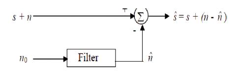
Adaptive filters are able to conform their drive reaction to channel out the associated flag in the information. They oblige next to zero from the earlier information of the sign and commotion attributes. On the off chance, the sign is narrowband and clamor broadband, which is generally the case or the other way around, earlier data is not required else they oblige a flag that is related in some sense to the sign to be assessed [1],[3]. Besides versatile channels have the ability of adaptively following the sign under non-stationary conditions. Commotion Cancellation is a variety of ideal separation that includes creating an evaluation of the clamor by shifting the reference data and afterward subtracting this commotion gauge from the essential information containing both flag and commotion as indicated in Figure 1.
Figure 1. Noise Marvel in Channel
It makes utilization of helper or reference information which contains a corresponded estimate of the clamor to be scratched off. The reference can be obtained by putting one or more sensors in the confusion field where the sign is missing or its quality is adequately weak. Subtracting bustle from the sign incorporates the risk of de-forming the sign and if done detestably, it may incite an addition in the commotion level. This obliges that the clamor gauge  ought to be a careful reproduction of n. On the off chance it was conceivable to know the relationship in the middle of n and , or the attributes of the channels transmitting commotion from the clamor source to the essential and reference inputs are known, it would be conceivable to make a close gauge of n by planning an altered channel. On the other hand, subsequent qualities of the transmission ways are not known and are capricious, sifting and subtraction are controlled by a versatile procedure. Subsequently, a versatile channel is utilized that is fit for modifying its drive reaction to minimize a lapse signal, which is subject to the channel yield. The change of the channel weights and the motivation reaction is administered by a versatile calculation. With versatile control, clamor diminishment can be fulfilled with little danger of bending the signal [3],[5] , [8].
Section 2 explains the need of system identification and echo cancellation of signals. Section 3 explains the adaptive filter implementations like LMS and NLMS algorithms. Results and discourses are in Section 4.
In the class of uses managing identification, a versatile channel is utilized to give a straight model that shows the best fit to an obscure plant. Here, same information is given to both the versatile channel and the plant. The yield of the plant will serve as the fancied sign for the adjustment process [1].
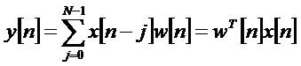
In this application, the obscure framework is displayed by a FIR channel with flexible coefficients. Both the obscure time –variant framework and FIR channel model are energized by an info arrangement u(n). The versatile FIR channel yield y(n) is compared with the obscure framework thay yields d(n) to create an estimation mistake e(n). The estimation blunder shows the contrast between the obscure framework yield and the model (evaluated) yield. The estimation mistake e(n) is then utilized as the data to a versatile control calculation which redresses the individual tap weights of the channel. This procedure is rehashed through a few emphasis until the estimation mistake e(n) turns out to be adequately little in some measurable sense [4],[8]. The resultant FIR channel reaction now explains about the beforehand obscure framework. It is demonstrated in Figure 2.
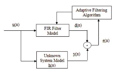
Figure 2. Model of System Identification
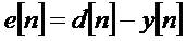
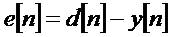
An Adaptive filters are element channels which iteratively modify their qualities to accomplish an ideal coveted yield. An Adaptive filter algorithmically adjusts its parameters keeping in mind the end goal to minimize a component of the differentiation between the look for yield d(n) and its bona fide yield y(n). This limit is known as the expense capacity of the versatile calculation. Figure 3 demonstrates the evil presence which states a square graph of the flex-ible reverberation wiping out framework. Here, the channel H(n) shows the motivation reaction of the acoustic environment, W(n) to the versatile channel used to scratch off the reverberation signal. The versatile channel plans to like its yield y(n) to the craved yield d(n) (the signal resonated inside of the acoustic environment). At every emphasis the slip signal, e(n) =d(n)-y(n), is bolstered over into the channel, where the channel attributes are changed in like manner [3],[7],[8].
The point of a adaptive channel is to ascertain the contrast between the wanted signal and the adaptive field yield e(n). This error signal is bolstered over into the adaptive filter and its coefficients are changed algorithmically keeping in mind the end goal to minimize an element of this distinction, known as the cost function. On account of acoustic reverberation wiping out, the ideal yield of the versatile channel is measured up to the undesirable echoed signal. At the point when the adaptive filter yield is equivalent to sought sign, the lapse signal goes to zero. In this circumstance, the echoed signal would be totally wiped out and the far client would not hear any of their unique discourse back from them [4].
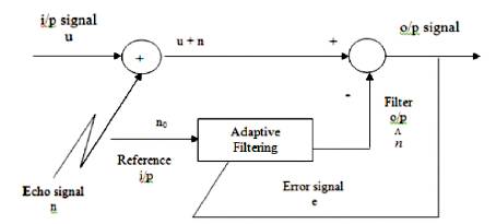
Figure 3. Versatile Reverberation Canceller Framework
LMS algorithm consists of three distinct steps in each iteration of this order:
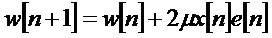
The principle explanation behind the LMS calculations notoriety in versatile sifting is its computational straight forwardness, making it less demanding to execute than all other normally utilized versatile calculations. For each weight, the LMS algorithm calculation obliges 2N increments and (2N+1) duplications[2].
As the step size parameter is picked in view of the present information values, the NLMS calculation demonstrates far more prominent security with obscure signs. This combined with the joining rate and relative computational straightforwardness makes the NLMS figuring ideal for the steady adaptable resonation fixing system.
As the NLMS is an increase of the standard LMS computation, the NLMS calculations practical utilization is close to the LMS count. In every cycle, the NLMS computation involves these movements, in the going with solicitation.
Every cycle of the NLMS calculation obliges 3N+1 duplications, this is just N more than the standard LMS calculation and this is a satisfactory build considering the increases in dependability and reverberation weakening accomplished [6].
Some essential measures will be examined in the accompanying areas. For example, convergence rate, MSE, computational multifaceted nature.
The Convergence rate decides the rate at which the channel unites to its resultant state. Typically, a quicker joining rate is a coveted normal for a versatile framework. Merging rate is not free of the various execution qualities. There is generally a tradeoff, with union rate and other execution criteria.
The MSE is a metric demonstrating the amount a framework can adjust to a given arrangement. A little MSE is an evidence that the versatile framework has precisely displayed, anticipated, adjusted and/or focalized to an answer for the framework. There are various elements which will help to focus the MSE including, yet not constrained to; quantization commotion, request of the versatile framework, estimation clamor, and slip of the inclination because of the limited step size.
Computational intricacy is especially essential for continuously versatile channel applications. At the point when a continuous framework is being executed, there are equipment constraints that may influence the execution of the framework. An exceedingly complex calculation will oblige much more noteworthy equipment assets than a shortsighted calculation.
LMS algorithm provides better minimum MSE. NLMS based adaptive filter provides better speed. LMS is chosen for denoising, a larger step size should be kept small, for NLMS step size should be smaller and the filter length should also be small. In the event, while merging execution of the standard LMS calculation to the NLMS variation, the NLMS calculation adjusts in far less cycle to an outcome on a par with the non-standardized calculation. The performance analysis parameters of LMS and NLMS algorithm are shown in Table 1. The LMS and NLMS Conversion Performances are shown in Figure 4.
Figure 4. Comparing the LMS and NLMS Conversion Performance
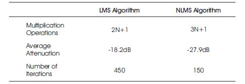
Table 1. Multiplication operations, Avg Attenuation and iterations of LMS and NLMS Algorithm
In this paper we conclude that, the LMS algorithm computational complexity is simple, which requires 2N+1 multiplication operations with average attenuation of - 18.2dB. NLMS algorithm requires multiplications of 3N+1 with average attenuation of -27.9 dB. In the considered problem, LMS requires approximately 450 number of iterations where as NLMS requires approximately 150 number of iterations. Hence, NLMS algorithm have faster convergence rate, a better steady state response than LMS and NLMS algorithm doesnot require a prior knowledge of the signal to certain stability. It was the observable alternative for real time applications.
There are many possibilities for further development in this discipline, One of these are as follows. Affine combination of two TVLMS adaptive filters can be used to avoid the slow convergence behavior and more robust variant and also it shows a superior harmony between the effortlessness and execution with the less tap size and iterations.