(1)
One of the most important problems in many application areas is to extract the signal of interest from background noise. In background noise, the occurrence of signal and the behaviour of signal are random. Therefore, it is reasonable to deal with the signal extraction problem using methods based on probability theory and statistical estimation. That is to say that signal detection and parameter estimation problems are statistical hypothesis testing problems in mathematical statistics. In this paper, we examine signal and noise environments encountered in active sonar using CW and LFM pulses. The optimum receiver is presented for range-Doppler-shift processing in a background-noise-limited environment. FFT based implementation for detection of CW and LFM active sonar target has been shown here. By following this method both range and Doppler resolution can be achieved.
SONAR (SOund NAvigation and Ranging) systems have many similarities to radar and electro- optical systems. The process of sonar is based on the propagation of sound waves between a target and a receiver. The main purpose of sonar is the detection or classification (estimation of position, velocity, and identity) of submerged, floating or buried objects. The nature of the required object known as the sonar target depends on the application. Examples include man-made objects of military interest (a mine or submarine), shipwrecks (as a navigation hazard or archaeological artifact) and fish (the target of interest to a whale or fisherman). In military applications, sonar systems are used for detection, classification, localization and tracking of submarines, mines or surface contacts as well as for communication, navigation and identification of obstructions or hazards (e.g., polar ice). In commercial applications, sonar is used in fishfinders, medical imaging, material inspection and seismic exploration [2].
The two most common types of sonar systems are passive and active. Passive sonar includes a receiver but no transmitter. The signal to be detected, then the sound emitted by the target. In an active sonar system, waves propagate from a transmitter to a target and back to a receiver, analogous to pulse-echo radar. In addition to these two types, there is also daylight or ambient sonar where the environment is the source of the sound which bounces off or is blocked by the target and the effects of which are observed by the receiver. This latter type of sonar is analogous to human sight [1].
Active sonars know more about the signal to be detected and therefore the receiver is designed to match the signal i.e., it uses matched filter processing. But the background against which the signal has to be detected contains reverberation in addition to the ambient and self-noise of passive sonar's [10]. This additional background is all important in active systems and the designer must be aware of its magnitude and how to discriminate against it. Active sonars employ two broad classes of pulse types. Continuous Wave (CW) is a pulse of constant frequency and duration T seconds. The bandwidth of the pulse, and of the matched filter for optimum detection of this pulse, is 1/T Hz. Frequency Modulation (FM) is the frequency of the pulse changed during the T second's duration of the pulse. The bandwidth B is not now the inverse of the pulse length [3].
Reverberation is mainly due to multiple reflections of the transmitted signal by the ocean surface ground and volume. So, the target detection of active sonar is difficult in the presence of reverberation. Statistical characterizations of reverberation noise are difficult to find out. To achieve a good performance against reverberation, the optimum centre frequency must be designed to maximize reverberation rejection [7][8][9]. By choosing proper optimum centre frequency we can reduce the effect reverberation on the transmitted signal. So, here in this paper the detector which is optimised in the background noise limited case is designed using FFT based implementation and attempt to minimize the effect of reverberation noise on performance. That is FFT based implementation for background-noise-limited environment [4][6] using linear frequency modulation (LFM) and continuous wave (CW) pulses are shown which gives both Doppler and range resolution.
Section 1 gives brief introduction about mathematical modelling of CW and LFM waveforms. Section 2 deals about how LFM and CW is processed in Range-Doppler shift. Finally, FFT based implementation is shown in section 3 and the simulation are shown in section 4 results.
Frequency or phase modulated waveforms can be used to achieve much wider operating bandwidths. Linear Frequency Modulation (LFM) is commonly used. In this case, the frequency is swept linearly across the pulse-width, either upward (up-chirp) or downward (down-chirp). Formula below shows a typical example of an LFM waveform. LFM can be mathematically written as
Where fo is the centre frequency,  and is the sweep rate.
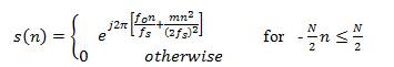
The idea of the ambiguity function and ambiguity diagram by considering the simple continuous wave (CW) pulse is illustrated, where s(n) is defined by
Consider the optimum detectors for the CW pulse in background noise limited environment. A statistical characterization of reverberation noise is necessary to derive the optimum detector in reverberation noise-limited environment [5][7]. Because of the problems in obtaining such a characterization in practice, the detector optimised for the background noise limited case and attempt to minimize the effect of reverberation noise on performance is often used. Parameters under the control of the design engineer are
Consider the CW pulse and. assuming that is operating in zero mean white Gaussian noise. The optimum detector is just the quadrature receiver shown below in Figure 1. The number of samples that is summed is set equal to the length of the pulse. The fact that the quadrature receiver is optimum detector is reasonable the problem of detecting sinusoidal signal of finite duration in noise.
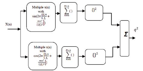
Figure 1. Quadrature receiver (number of samples summed equals to the length of the LFM pulse)
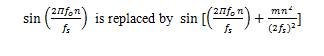
For the LFM pulse the optimum detector has the same form as the quadrature receiver with the exception that
This is why we are the correlating the received signal with stored replica of the LFM pulse.
That is, the received signal with a store replica of the LFM pulse is correlated. Quadrature receiver is shown in Figure 1.
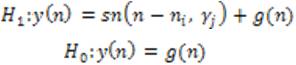
Now involving two variables the hypotheses are
The composite receiver consists of the set of optimum detector, adjusted to the discrete frequencies, yj, and j=1……….J calculated at a set of discrete time, ni, i=1, 2 ...I. At each value of ni the maximum output of J detectors is compared to the threshold. If the maximum output exceeds the threshold, the frequency value to which the detector is matched serves as the estimation of γ, or Doppler shift. The time at which the detection occurs is the estimate of range.
Optimum detector is a quadrature receiver shown in Figure 2. A bank of such detectors is implemented in parallel, where each detector is adjusted to a separate frequency, ,  The output of the detectors is calculated at a time intervals n1,n2 ,.....ni. At ith time, the output of the jth optimum detector is given by,
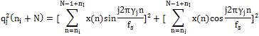
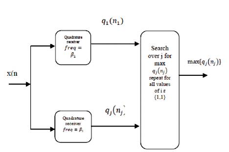
Figure 2. Implementation of the multiple alternative hypotheses test for range and Doppler shift
The implementation of multiple alternative hypotheses are shown in Figure 2.
The global maximum over the indices i and j in the previous equation provides the estimates of the range and Doppler shift. A DFT followed by an SLD for each frequency bin, is approximate realization of quadrature receiver is shown in Figure 2. The length of the DFT is matched to the duration of the pulse.
Consider a set of CW with the centre frequency of 3 Hz. The lengths of the pulses ranging from 5ms to 1s are considered. By using these set of pulse lengths the effect of reverberation noise pulse for contacts with various values of Doppler shift are minimised. The maximum velocity is assumed as 30 knots in magnitude and c as 3000 knots. The compression parameter at maximum v, ,  will fall in the range of -0.02δ ≤ 0.02. Therefore the maximum Doppler shift magnitude is equal to 60Hz.
To obtain an FFT based implementation for 62.5 to 1000ms pulses. the frequency width varies inversely with T where it achieves a maximum value of 32Hz for the 62.5ms pulse. As a result of Doppler shift, the received centre frequency occurs in the range of fo - 60≤ f ≤ fo+ 60. After shifting the centre of spectrum to zero frequency, the highest frequency in the baseband data is given by 76Hz. Selecting a sampling frequency of 256Hz at the input to the FFT results in a transition region for the low pass filter, fa-fp is equal to 104Hz. The highest frequency in the analog data is equal to the sum of the normal centre frequency maximum Doppler shift and half of the maximum/power spectral width. Therefore, the highest frequency in the analog signal is 3260 Hz. If aliasing is allowed in the transition region of analog filter, then a sampling frequency of 8192Hz results in transition region of fp /(fs -fp ) is equal to 0.66. This corresponds to use of a 6-pole 6-zero elliptic antialiasing filter. It is desirable to use a short analog filter by over sampling the analog filter to 16384Hz. This is given to the square law detector. The output is compared with threshold to detect whether the target is present or not. The length of the FFT is given by Tfs which is equal to 265. The FFT length to the pulse length is matched [4].
Consider a set of LFM with the centre frequency of 3 Hz and lengths ranging from 5ms to 1s. Consider sweep extent is 200Hz. Such a set of pulse lengths allows us to minimise the effect of reverberation noise pulse for contacts with various values of Doppler shift. Let the maximum velocity is 30 knots in magnitude and c=3000 knots, the component parameter at maximum v will fall in the range of -0.02≤δ≤ 0.02. Therefore maximum Doppler shift is equal to 60Hz. Obtain an FFT based implementation for 62.5 to 1000ms pulses. The frequency width varies inversely with T, it achieves a maximum value of 32Hz for the 62.5ms pulse spectral width. As a result of Doppler shift (60Hz as derived above), the received centre frequency occurs in the range of fo -60≤ f ≤ fo +60. After shifting the centre of spectrum to zero frequency, the highest frequency in the baseband data is then 60+32/2=76Hz.
Selecting a sampling frequency of 256Hz at the input to the FFT results in a transmission reason of the LPF of fa-fp=(256- 76)-76=104Hz. Such a transition region is provided by FIR filter of reasonable length. To establish the sampling frequency for ADC, we note that the highest frequency in the analog data is equal to the sum of the normal centre frequency, the maximum Doppler shift and half of the maximum power spectral width. The 5 milliseconds pulse has a spectral width of 400Hz centred. Therefore, the highest frequency in the analog signal is 3260 Hz. If aliasing is allowed in the transition region of analog filter, a sampling frequency of 8192Hz resulting in transition region of fp/(fs-fp) will be 0.66. This corresponds to a 6-pole 6-zero elliptic anti aliasing filter. It is desirable to use a short analog filter by over sampling the analog filter 16384Hz. The length of the FFT is given by Tfs=265. We thus have matched the FFT length to the pulse length. The signal processing for the LFM is shown in Figure 3.
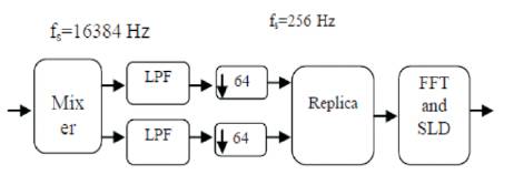
Figure 3. Signal processing for the LFM and CW pulses
The transmitted CW pulse of frequency 3 kHz, the delayed and Doppler shifted signals of PSD, are also shown in Figures 4 and 5. The sampling frequency is 16384 kHz. Pulse width is 62.5ms. Number of samples is 1025 samples. Figure 6 shows received signal with White Gaussian Noise. The inphase and quadrature-phase components after decimation are shown in Figure 7, Figure 8 shows PSD of receiver output inphase and outphase components after filter.
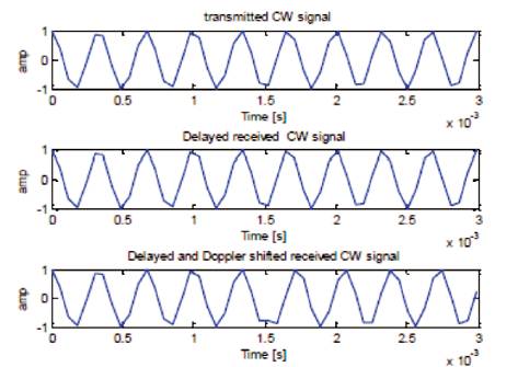
Figure 4(a) Transmitted CW signal, (b) Delayed received CW signal, (c) Delayed and Doppler shifted received CW signal
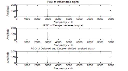
Figure 5(a) PSD of Transmitted CW signal, (b) PSD of Delayed received CW signal, (c) PSD of Delayed and Doppler shifted received CW signal
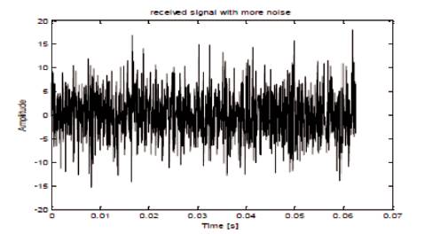
Figure 6. Received Signal With White Gaussian Noise
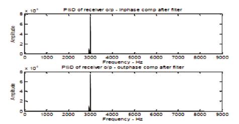
Figure 7. PSD of receiver output inphase and outphase components after filter
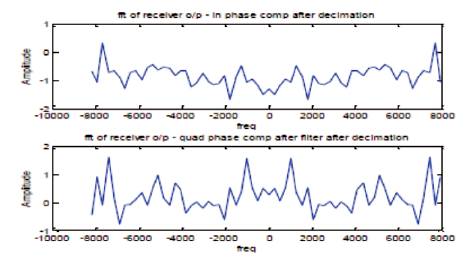
Figure 8. PSD of receiver output inphase and outphase components after filter
The transmitted LFM pulse of frequency 3 kHz, the delayed and Doppler shifted signals of PSD, are also shown in Figures 9 and 10. Consider the sampling frequency as 16384Hz, centre frequency as 3 KHz, velocity of sound as 1500m/s, chirp bandwidth as 1000Hz, chirp pulse width as 62.5 ms, and number of samples as 1025. Assuming that the target is present at 8000m, the following results are obtained using MATLAB. The results shown below are the outputs of each block of Figure 3. Then the output of the Square Law Detectors (SLD) shown in Figure 13 is compared with the threshold in order to detect that the target is present or not. Figure 11 and 12 shows Received Signal with White Gaussian Noise and PSD of receiver output inphase and outphase components after filter.
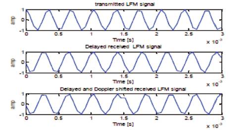
Figure 9(a) Transmitted LFM signal, (b) Delayed received LFM signal, (c) Delayed and Doppler shifted received LFM signal
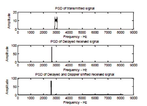
Figure 10(a) PSD of Transmitted LFM signal, (b) PSD of Delayed received LFM signal, (c) PSD of Delayed and Doppler shifted received LFM signal
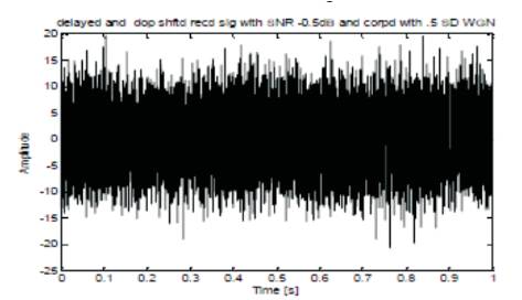
Figure 11. Received Signal with White Gaussian Noise
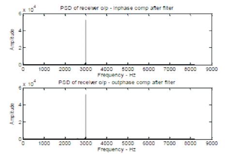
Figure 12. PSD of receiver output inphase and outphase components after filter
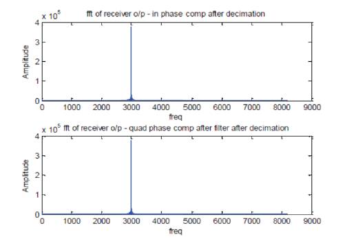
Figure 13. FFT of receiver output inphase and outphase components after filter after decimation
The FFT based implementation of LFM and CW active sonar under noise background environment is implemented using MATLAB successfully and the results are shown. The threshold using Neyman-Pearson (NP) criterion is found out. The maximum output of the detector is compared to that threshold in order to detect the target presence. The target presence is shown in command window. FFT of received Doppler shift signal is shown. The resolution of the FFT is as fine as 3-dB Doppler shift intercept of the ambiguity diagram. At output of the filter, the length of the FFT is given by T fs = 265.