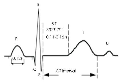
Figure 1. ECG Wave of a Heart Beat
The cardiovascular diseases such as Arrhythmia and Myocardial Infarction are becoming more alarming in causing heart attacks. The early detection of cardiac related deceases has become an essential activity to save a patient from death. For detecting these cardiovascular diseases useful information is hidden in the ECG waves, and it has to be extracted from the ECG signal. In this paper the authors used the Hilbert Transform (HT), Principle Component Analysis (PCA) and Independent Component Analysis (ICA). The Hilbert Transform is useful in providing good resolutions to the ECG and it is able to easily interpret the unknown difficulties in the ECG. The Principal Component Analysis (PCA) and Independent Component Analysis (ICA) were independently applied on Hilbert Transformed ECG signal to enhance the hidden complexities in ECG signal by eliminating non-Gaussian noise elements. Later the suitable algorithms were applied to detect the fiducial points such as PQRST and perform statistical analysis on ST Interval variability. The authors have noted that the ICA has better performance than the PCA.
Electrocardiogram (ECG) is a waveform which represents the transthoracic interpretation of the electrical activity of the heart over time. A set of surface electrodes is used to measure the cardiac potential of the heart, and this cardiac potential can be correlated with regions of cardiac excitations, heart rate, and cardiac arrhythmias. In some occasions the electrical activation that is producing the normal heartbeat can cause abnormal cardiac function and disorders such as bradycardia (slow heart rate), tachycardia (fast heart rate) and bundle branch blocks. This makes the situation emand early diagnosis of the diseases from the reading of the ECG.
In 2005, L. Khadra et.al, (L. Khadra, A. S. Al-Fahoum, and S. Binajjaj) proposed a high order spectral analysis technique for quantitative analysis and classification of cardiac arrhythmias. Bispectral analysis techniques were used in the algorithm. In 2006, F. de Chazal et.al, (F. de Chazal and R. B. Reilly) proposed an efficient system to detect the premature ventricular contraction from diseased subjects. Three modules namely denoising module, feature extraction module and classifier module were used in this system. In 2006, S. Mitra et.al., (S. Mitra, M. Mitra, and B. B. Chaudhuri, 2006) introduced a three stage technique to detect Premature Ventricular Contraction (PVC) from normal beats and other heart diseases. A novel approach of ECG classification was presented by Nazmy et al., (T. M. Nazmy, H. El-Messiry and B. Al-bokhity) in 2009. In this paper an intelligent diagnosis system by using hybrid approach of Adaptive Neuro-fuzzy Inference System (ANFIS) model was used for classification of Electrocardiogram (ECG) signals. In 1999, I. Christov and I. K. Daskalov, proposed a method to approximate filter characteristics dynamically depending on the ECG signal slope. In this procedure the slope is evaluated despite the EMG noise component. A novel procedure was presented by Yue-Der Lin and Yu Hen Hu, detect and suppress interference of power line (PLI) from ECG signals. In 1985, the European Community initiated an action to standardize the approach to detect and interpret ST segment and T-wave changes. In 1988, Aldrich developed an ECG score based on ST-segment deviation to quantify the size of the total risk in acute Anterior and Inferior Myocardial Infarction (AMI). In 2009, Erik Zellmer presented a highly accurate ECG beat classification system to form three separate feature vectors from each beat by using the combination of Continuous Wavelet Transformation (CWT) and time domain morphological analysis. In 2010, Philip Langley used Principle Component Analysis (PCA) for analyzing changes in ECG morphology and for the derivation of surrogate respiratory signals from single-lead ECGs.
The ECG is used as a diagnostic tool to identify the cardiac deceases by interpreting the details that it contains. Figure 1 shows the ECG wave with all the important information pertaining to the patient's heart condition. It has P wave, QRS complex and T wave [1]. The QRS complex and T wave are having the same direction with duration about 0.05- 0.25 seconds. T wave takes up a longer time and has amplitude of one tenth of that of R wave. The Table 1 demonstrates briefly the important features of ECG signal [2]. The heart has four chambers and each chamber performs a different part of the circulatory process mentioned in Figure 2.
Figure 1. ECG Wave of a Heart Beat
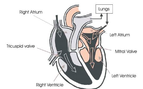
Figure 2. Structure of the Human Heart
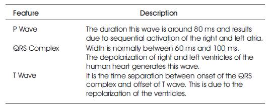
Table 1. ECG Characteristics
The heart pumps the oxygenated blood from the lungs to the body parts through the arteries and collects deoxygenated blood back to the lungs from the body through the veins. A sequence of events occurs in a specific order called the cardiac cycle. The cardiac cycle has two phases namely systole and diastole. Diastole phase is when the heart muscle is relaxed and begins to fill with venous blood in the right atrium and oxygenated blood in the left atrium. Systole is the time when the heart contracts. During systole the oxygenated blood is forced out of the left ventricle and deoxygenated blood is forced into the lungs through the right ventricle. Deoxygenated blood first enters the heart via the superior and inferior vena cava and fills the right atrium. As the atria contracts this blood is pumped into the right ventricle. After blood fills the right ventricle it contracts to pump venous blood into the lungs. After this blood is purified the oxygenated blood then returns to the heart via the pulmonary vein and fills the left atrium. Later the left atrium contracts and sends the blood into the left ventricle.
As the left ventricle is filled up it contracts and pumps the oxygenated blood out of the heart through the aorta. The electric conduction system of the human heart is shown in the Figure 3.
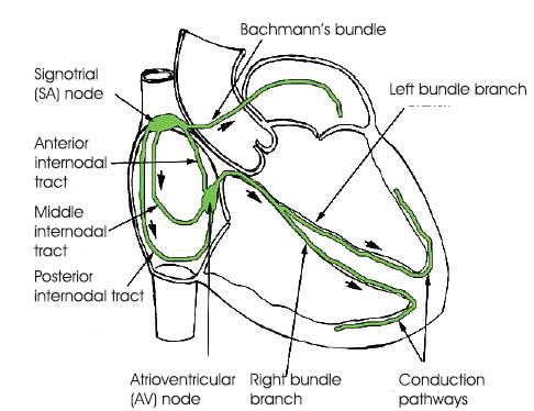
Figure 3. Conduction System of the Human Heart
The cardiac cycle of diastole and systole is controlled by electrical conduction system consisting of the SA node, AV node, branch bundles, bundle of his conduction paths. SA node acts as natural pacemaker of the heart and generates the electrical impulses to regulate the cardiac cycle. The electric impulses spread from the SA node via the internodal fibers of the right atrium, and then to the left atrium, causing immediate atrial contraction. This electrical potential travels to the AV node and then gets delayed to allow the atria to fully contract. This allows the atrium to empty its contents completely into the ventricles before ventricular contraction. From the AV node, the potential travels down the Bundle of His and splits into the right and left branch bundles which innervate the ventricular walls via the Purkinje fibers. Finally the potential reaches the Purkinje fibers and controls ventricular contraction. This process repeats for the next heartbeat.
The Hilbert transform of a real time function s(t) is defined as:
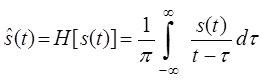
If the integral exists, the independent variable will not change as a result of this transformation, so the output is also a time dependent function [3][4]. Since there a possibility of a singularity at τ = t it is not possible to determine the Hilbert transform as an ordinary improper integral. The integral is then to be considered as a Cauchy Principal Value. In mathematics, the Cauchy principal value of a certain function is defined as
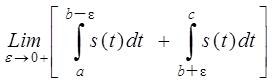
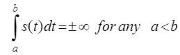
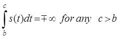
Where b is a point at which the behavior of the function s(t) is such that
If the Hilbert transform exists, it can be written as given in (1). The Hilbert transform can also be written as a convolution of 1/πt and s(t) and expressed as:
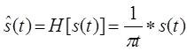
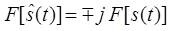
Equation (5) shows that is a linear function of s(t). The frequency domain representation of (5) is obtained as the product of their Fourier Transforms, Fourier of two functions with help of the convolution theorem and is treated as the spectrum of H[s(t)]. Mathematically the spectrum is represented as:
Therefore the Hilbert transform is equal to – j for positive frequency and + j for negative frequency. Hence it is equivalent to a filter, in which the every frequency component is allowed to pass without any attenuation but their phases are altered by -П/2 radians or +П/2 radians depending upon the sign of the frequencies. Finally the Fourier transform of the Hilbert transform of s(t) is given by
One of the linear dimensionality reduction procedures which seeks the projection of the data into the directions of highest variability is Principal Component Analysis (PCA) [5]. It computes the principal components which are the basis functions of directions in decreasing order of variability. The basis functions in Fourier Transform are predefined and assumed to be independent, whereas in PCA the basis functions are found in the data by looking for a set of the basis functions that are independent. That is, by using variance as the metric, the data undergoes a decorrelation. The second order basis functions are independent as these are orthogonal (the dot product of the axes, and the cross-correlation of the projections are close to zero).
The first principal component gives basis functions in the direction of highest variability. The second principal component provides the basis vector for the next direction orthogonal to the first principal component and so on. A threshold is set to the percentage of total variability of the data in order to select the number of principal components. Calculation of principal components involves calculation of covariance matrix of the data, its eigenvalue decomposition, sorting of eigenvectors in the decreasing order of eigenvalues and finally projection of the data into the new basis defined by principal components by taking the inner product of the original signals and the sorted eigenvectors. The comprehensive procedure of PCA is presented below:
Step 1: Computing the covariance matrix from the data as;
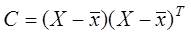
Where X is the data matrix of Hilbert Transformed ECG signal and represents the mean vector of X.
Step 2: Computing the matrix of eigenvectors V and diagonal matrix of eigenvalues D as;
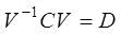
Step 3: Sorting the eigenvectors V in the descending order of eigenvalues in D and then the data is projected on these eigenvector directions by taking the inner product between the data matrix and sorted eigenvector matrix as;
Projected data
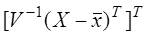
The six features for subsequent classification are the first six columns of the projected data. The six components were selected based on availability of 99% of the total variability.
It is one of the Blind Source Separation Technique. ICA is used to identify and separate mixtures of sources with little prior information. ICA is distinguished from other methods as it looks for components that are both statistically independent and non Gaussian. In particular let us consider ECG, which is a mixture of signals from nodes presented in the heart and various artifacts and noise. Basic ICA model assumes linear combination of source signals (called components) [6][7]

Where X, S are the two vectors representing the observed signals and source signals respectively and A is an unknown matrix called the mixing matrix. Mixture matrix A size n x n (in general A does not need to be square, but many algorithms assume this 'property'), X and S get the size of n x m, where n is number of sources and m is length of record in samples. Incidentally, the justification for the description of this signal processing technique as blind is that we have no information on the mixing matrix, or even on the sources themselves. The objective is to recover the original signals, S, from only the observed vector X. Denoting the output vector by V, the aim of ICA algorithms is to find a matrix U to undo the mixing effect [8]. That is, the output will be given by

Where, V is an estimate of the sources. The sources can be exactly recovered if U is the inverse of A up to a permutation and scale change.
The BSS/ICA methods try to estimate components that would be as independent as possible, and their linear combination is original data. Estimation of components is done by iterative algorithm, which maximizes function of independence, or by a non-iterative algorithm, which is based on joint diagonalization of correlation matrices, [9][10]. ICA has one large restriction that the original sources must be statistically independent. This is the only assumption we need to take into account in general. The reconstructed ECG can be derived by using the following equation

Where, V is the matrix of derived independent components with the row representing the noise or artifacts set to zero. After getting ICs it is necessary to determine the order of the independent components in order to identify normal ECG, noise and abrupt alterations. As the ICs corresponding to noise and abrupt alterations have more distinctive properties than that of original signal both in time and frequency domains, we may employ the statistical properties of these waveforms to recognize the original ECG automatically instead of identifying visually. The noise is identified by using kurtosis and abrupt changes by using variance. The kurtosis is the fourth order cumulant. For a signal x(n), it is classically defined as in (16) by dropping n for convenience

Here the kurtosis is zero for Gaussian densities. The normal ECG will have large Kurtosis value than continuous noise. In their approach, a threshold was chosen from analysis of sample waveforms, and a component whose modulus of kurtosis is below this threshold will be considered as continuous noise.
The variance or energy is more or less similar and negligibly small for all IC waves except for those IC waves containing abrupt changes. Thus the IC waves whose variance is large can be identified as abrupt variations or noise. The variance of signal x(n) is given by
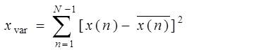
Where is the mean value of x(n).
The proposed method is described in Figure 4. First the original ECG signal is preprocessed with a lowpass filter with a cutoff frequency of 45 Hz to remove the high frequency noise and motion artifacts. Next the ECG is passed through a highpass filter designed to a cutoff frequency of 0.05 Hz to remove the baseline wander. A notch filter is designed to remove powerline interference component from ECG.
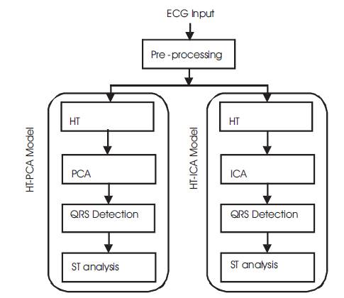
Figure 4. Proposed Method of ECG Analysis
In this proposed model the combination of HT and PCA is used on preprocessed ECG signal to remove Gaussian noise present within the passband of the ECG signal. Next PCA is applied on the HT processed ECG to get PCA components. For evaluating the signal improvement, the correlation coefficient between the noise-free signal and the output after PCA filtering was computed. In addition, Signal to Noise Ratio (SNR) before and after PCA filtering was estimated. SVD (Singular Value Decomposition) algorithm is used for finding PCA components. Then, the PC's were sorted in descending order based on their correlation coefficient. Next, the Principal Components (PC) with highest variance for high SNR (over 0 dB) are selected and the PCA projection is inverted. The median and Median Absolute Deviation (MAD) values over all the ECG leads were considered as representative values for each signal. As median and MAD are more robust to outlier values, they were preferred to the arithmetic mean and standard deviation. This analysis is performed by using Singular Value Decomposition (SVD) algorithm.
In proposed HT-ICA model approach, the modulus of Kurtosis value of each ICA component is evaluated and compared with the threshold. If the modulus of Kurtosis exceeds the threshold, that IC is marked as continuous noise component. Then, the remaining ICA components are divided into 10 non overlapping blocks, each of onesecond duration. The variances of the 10 segments for each component are calculated as shown in (17), and then the variance of these 10 variance values is obtained as the parameter xvar. The component whose xvar value is above a predetermined threshold is marked as an abrupt change component. Finally, the required ECG can be obtained using (14) and (15). This analysis is performed by using JADE algorithm.
After the ECG processed in both approaches, the ECG is operated with simple QRS detection algorithm. Extracted ECG is differentiated to get a new signal which is proportional to slope. QRS complex is enhanced by transforming each QRS complex into single positive peak by squaring and integrating with moving window. By setting a threshold the R-peak is determined first and later Q and Speaks are determined by searching backward and forward from R-peak. Next, the ST episodes are identified after finding the fiducial points. The time separation between J point and K point is known as ST segment. [11][12]. The J point is located after S peak where the slope of the ECG is flattest. In the case of tachycardia (HR > 60 beats/sec) the K point is located at 40 ms after J point. In case of bradycardia (HR < 60 beats/sec) the K point is located at 80 ms after J point. From the J point and K point the ST interval is measured. These values are in general agreement with the recommendation of the European ST-T database.
The authors tested their proposed method on MIT-BIH Long Term ST database. One ECG record 's20041m' taken from the MIT-BIH Long Term ST database and preprocessed by using Hilbert Transform and then processed with PCA by using SVD (Singular Value Decomposition) and ECG extracted. Later QRS detection algorithm was applied on purified ECG to determine first R peak and the Q & S peaks. Similar steps were followed after ICA is applied on Hilbert Transformed ECG. In both cases ST interval is measured. The ECG wave taken from Physionet database is shown figure 5. The PCs and ICs are shown in the Figure 6 and Figure 8. Finally the ECG with identified peaks in both case are shown in Figure 7 and Figure 9.
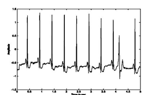
Figure 5. The ECG from MIT-BIH Database
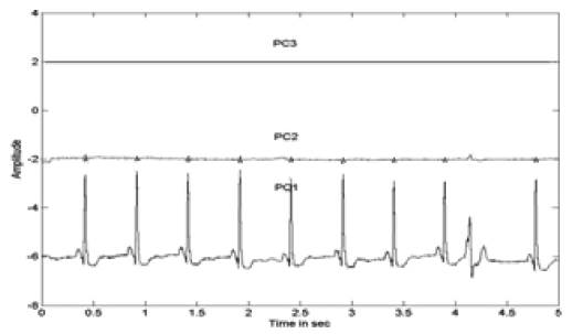
Figure 6. Extracted PCs of the ECG
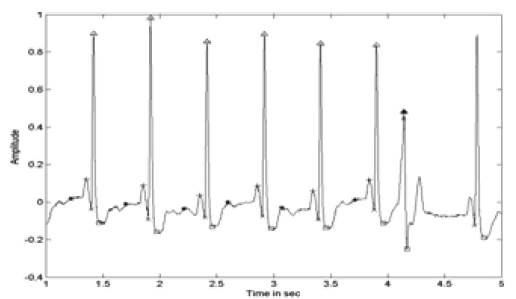
Figure 7. ECG with Identified PQRST Points After PCA
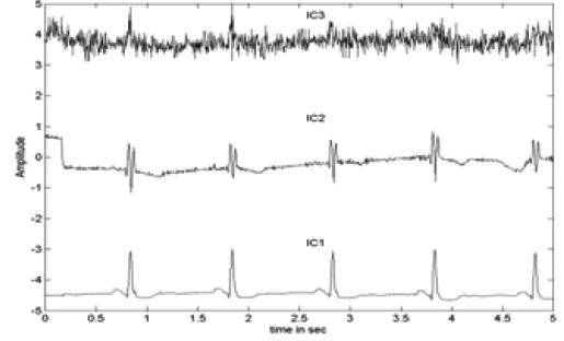
Figure 8. Extracted ICs of the ECG
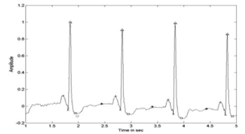
Figure 9. ECG with Identified PQRST Points After ICA
In transform domain the hidden complexities in the ECG signal were visible more clearly than the conventional time domain. Moreover with the HT on the signal, more futuristic characteristics can be enhanced. When the dimensionality reduction method was applied on an ECG signal, the features would contain a compact representation.
When these features were identified by simple and well QRS detection algorithm, it is simple and would result in higher accuracy. Two commonly used dimensionality reduction methods, PCA and ICA were used to reduce the dimensionality. The aim of investigating various dimensionality reduction techniques was accomplished through the support of the Hilbert Transform as discussed in this paper.