As the satellite transmissions at C band and Ku band become more congested, it will be necessary to use higher frequency bands for additional services. At present new services are being introduced in the Ka band. None of the accessible International Telecommunications Union (ITU) models are validated for predication attenuation in the accepted manner and hence it calls for a new propagation experiment to validate the accessible models and comes out with more suitable and accurate models to have a certain Quality of Service (QoS). Propagation experiment at this new band is necessary for the characterization of the various tropospheric phenomena which can degrade the transmitted signal. These measurements allow the development of new accurate tropospheric propagation models. Satellite beacons are frequently available for large antennas and can be used for measuring rain attenuation and other phenomena such as tropospheric scintillation. The designed receiver is established with 1.2 m antenna system to receive onboard GSAT 14 beacon at 20.2 GHz.

Ka band propagation studies testing have been conducted by different countries (Prakash et al., 2013; Prakash et al., 2009), where the study is related to their frequency and mode of procedure. The Digital Beacon Receiver is based on sensitivity and large dynamic rage. The Ka band beacon receiver design and RF front end design was proposed. The digital receiver is based on closed loop structure between Low Noise Block Convertor (LNBC) and L-Band Down convertor (LBDC) by using Keysight technology Advanced Design System software to estimate signal strength of the beacon signal.

In these techniques, the receiver utilizes the two beacon signals at 20.2 GHz and 30.5 GHz frequency using down converter with diving and conquers approach for achieving better accuracy during weak signal. The receiver is designed by ADS software schematic window. The designed simulations are HB simulation, S-Parameter simulation, AC simulation, Power Budget analysis, and Fast Fourier Transform (FFT) design at -110 dBm input power taken from downlink calculations. This work is essential to estimate signal strength of the beacon signal and the simulation results match with 98% of testing results.

The authors have designed an inexpensive Digital Beacon receiver system with two beacon signal at 20.2 GHz and 30.5 GHz frequency. The dual polarization (V and H) of single antenna structure with low noise down converter and Digital Beacon receiver design was simulated by using Advanced Design System (ADS) software to estimate the signal strength of the beacon signal. Satellite beacons are frequently available and designed for large antennas and can be used for measuring rain attenuation and other phenomena such as tropospheric scintillation. The act of the receiver system has been considered for dissimilar input power levels by using various simulation techniques, such as Harmonic Balance, S-parameter simulation, and Power budget Analysis, AC Simulation, and Digital Beacon Receiver with FFT. The tested results match with the simulated results. The dynamic range of the receiver system is identified with help of AC simulation. Experimental results are measured with help of spectrum analyzer at 70 MHz frequency of both Co-Polar and Cross- Polar. The simulated results with corresponding output waveforms are analyzed.

The information carrying ability of any radio satellite communication link is determined by the Radio Frequency (RF) power at the receiver input (Pratt et al., 2003).

Link Equation is given by,

where
P = Received Power r
G = Received Antenna Gain r
EIRP = Effective Isotropic Radiated Power
L = Path Loss of Antenna

2.1 Digital Beacon Details

There are two beacons set up onboard GSAT-14 satellite, which gives the two frequency signals with two polarizations as shown in Table 1.

Table 1. Digital Beacon Details

The block diagram of Ka band Digital Beacon Receiver is shown in Figure 1. The beacon signals are received form GSAT-14 satellite. The receiver consists of 1.2 m antenna, LNBC, LBDC, Digital Receiver and Signal Processing (DRSP) unit, and storage and display segment (PC). The antenna section consists of antenna, feed, Ortho Mode Transducer (OMT), and Diplexer. The same antenna receives the frequencies from both polarizations (Sharma, 2010).

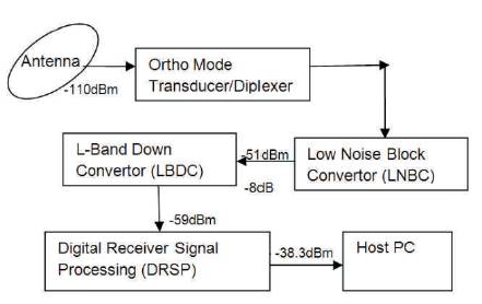
Figure 1. Block Diagram of Both Vertical and Horizontal Polarization of Digital Beacon Receiver (DBR)

The diplexer and OMT will divide both frequencies and polarizations. The LNBC’s input power is -110 dBm with frequency of 20.2 GHz, the local oscillator frequency is 19.2 GHz and the related Intermediate Frequency (IF) is 1 GHz. The 1 GHz frequency is given to input of LBDC and local oscillator frequency 930 MHz, the related Intermediate Frequency (IF) is 70 MHz. The 70 MHz Intermediate Frequency is given as input to the digital receiver and signal processing system and estimates the signal strength of the beacon signal are estimated.

The harmonic balance method is iterative. It is based on the statement that for a given sinusoidal excitation, there exists steady-state solutions that can be approximated to acceptable accuracy by means of a finite Fourier series. Accordingly, the circuit node voltages were taken on a set of amplitudes and phases for all frequency components (Keysight Esso EDA). The currents flowing from nodes into linear elements, including all circulated elements, are calculated by means of a straightforward frequencydomain linear analysis. Currents from nodes into nonlinear elements are calculated in the time-domain. Generalized Fourier analysis is used to transform from the time-domain to the frequency-domain. Digital receiver is simulated with help of Harmonic Balance (HB) simulation. The input power is around -110 dBm with frequency of 20.2 GHz as shown in Figure 2. If more than one fundamental is entered, the maximum mixing order is set. This limits the number of mixing products to be considered in the simulation. For more information on this parameter, see “Harmonics and Maximum Mixing Order” section under ADS HB Simulation. The simulation parameter is shown in Table 2.

Table 2. Simulation Parameters

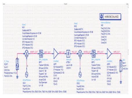
Figure 2. Block Diagram of Digital Receiver

The HB simulation consists of non-harmonically consistent sources and estimates the magnitude and phase of voltages or currents in a potentially nonlinear circuit. The techniques are:

• Compute quantities such as P dB, Third-Order 1 Intercept (TOI) points, Total Harmonic Alteration (THA), and intermodulation alteration components.
• Execute power amplifier and load-pull contour analyses.
• Carry out nonlinear noise analysis.
• Simulate oscillator harmonics, phase noise, and amplitude confines.

4.1 Simulation Results

The input power -110 dBm is passed through mixer_1 along with local oscillator 1 19.2 GHz with conversion loss of 4 dB. The output is -113 dBm as shown in Figure 3(a).

Figure 3. (a) Simulated Output of (Mixer1_Out)

Mixer 1 output is passed through Bandpass filter 1 having center frequency 1000 MHz with insertion loss of 1dB. The output is -114 dBm as shown in Figure 3(b).

Figure 3. (b) Simulated Output of (BPF1_Out)

The Bandpass filter 1’s output goes through low noise amplifier gain 1 of 60 dB with noise figure of 1.1 dB. The output is -55 dBm as shown in Figure 3(c).

Figure 3. (c) Simulated Output of (Amp1_Out)

The amplifier 1 output is passed through attenuation loss 8 dB. The output is -63 dBm as shown in Figure 3(d).

Figure 3. (d) Simulated Output of (PAD1_Out)

The pad loss is passed through mixer 2 long with local oscillator 2 930 MHz with conversion loss of 5 dB. The output is -67 dBm as shown in Figure 3(e).

Figure 3. (e) Simulated Output of (Mixer2_Out)

Mixer 2’s output is passed through Bandpass filter 2 having center frequency 70 MHz with insertion loss of 1 dB. The output is -68 dBm as shown in Figure 3(f).

Figure 3. (f) Simulated Output of (BPF2_Out)

The Bandpass filter 2’s output goes through the amplifier gain 2 of 30 dB with noise figure of 1.1 dB. The output is -39 dBm as shown in Figure 3(g).

Figure 3. (g) Simulated Output of (Amp2_Out)

S-parameter is used for the signal-wave response of an nport electrical element at a given frequency. It measures incident, reflected, and transmitted power and provides a l i n e a r S - p a r ame t e r, l i n e a r n o i s e p a r ame t e r s transimpedance, and transadmittance (Nandakumar et al., 2015). The simulation shows a 70 MHz center frequency as shown in Figure 4. S-parameter simulation normally allows:

Figure 4. Block Diagram of S-Parameter Simulation

• S11 - Forward Reflection (input match - impedance)
• S22 - Reverse Reflection (output match - impedance)
• S21 - Forward Transmission (gain or loss)
• S12 - Reverse Transmission (leakage or isolation).

The simulation frequency involves mixer sub-networks and enables AC frequency conversion, where the simulator causes the frequency of the source and mixer sidebands. Only the upper or lower sidebands are considered but not both.

5.1 Simulated Result

The two amplifiers are having a gain of 60 dB and 30 dB and the total gain is 90 dB and adding mixer conversion gain is 4 dB and 5 dB, Band pass filters have 1 dB each, and pad loss is 8 dB. The overall gain (S21) of the receiver is 70 dB at 70 MHz intermediate frequency (IF) based on the input signal level as shown in Figure 5

Figure 5. Simulated Output of S-Parameter

An AC simulation also offers a linear noise simulation option that can include the following noise contributions in its simulation:

• Temperature-dependent thermal noise as of lossy passive elements, including those particular by data files.
• Temperature and bias-dependent noise from nonlinear strategy.
• Noise from linear active devices is found to be meticulous by two-port data files that contain noise parameters.
• Noise from noise basis elements.

The noise simulation generates the noise affects and noise properties of the network. AC controller is used to carry out a swept-variable small-signal linear AC simulation.

We can simulate a single Frequency point, or across a frequency distance in a linear or logarithmic sweep simulated at 1GHz frequency using the model as shown in Figure 6.

Figure 6. Block Diagram of AC Simulation

6.1 Simulation Result

The graph is drawn between freq (GHz) vs. dBm (Amp2_out). In this simulation, the amplifier gains are 90 dB, insertion loss is 2 dB, and attenuation loss is 8 dB. The output is -31 dBm at 1 GHz as shown in Figure 7.

Figure 7. Simulated Output of AC Simulation

The output power variable with input powers from -110 dBm to -140 dBm at 1 GHz intermediate frequency as noted in Table 3 through simulation using ADS software.

Table 3. Output Powers for Different Input Powers

The power budget controller includes the power, Third Order Intercept, Gain and Noise figure measurements and this analysis is based on using frequency domain characteristics (Dunleavy et al., 1997; Bahri et al., 2014). The components may also contain mixers and nonlinear amplifiers. The analysis is performed at the double RF tone through specified power from the input signal -110 dBm source as shown in Figure 8.

Figure 8. Block Diagram of Power Budget Analysis

The budget is very useful to characterize the system behaviour and analyze the signal transitions from each component.

7.1 Simulation Results

A small power budget analysis signal is useful to evaluate the power flow through the system. The schematic representation of the Budget system is used in this simulation process as shown in Figure 9(a). The ADS schematic of an output power includes all necessary information as in Table 4.

Figure 9. (a) Power Budget for Output Power

Table 4. Power Budget for Output Power

This shows the simulation results for a single frequency of 1000 MHz. The first mixer along with local oscillator in the simulation is used to set the input power to the system during measurement, but is not part of the receiver itself. Hence the input power to the system is -110 dBm. The graph is drawn between Cmp_RefDes vs. Outpwr_dBm as shown in Figure 9(b).

Figure 9. (b) Power Budget for Component Noise Figure

The tabular column represents the Noise figure component of each block output as shown in Table 5.

Table 5. Power Budget for Component Noise Figure

The ADS schematic that includes all necessar y information is presented in Table 6. This shows the simulation results for a single frequency of 70 MHz. The graph is drawn between Cmp_RefDes vs. Outpgain_dB as shown in Figure 9(c).

Table 6. Power Budget for Gain in dB

Figure 9. (c) Power Budget for Component Noise Figure

The tabular column represents the output power budget for gain in each block output as shown in Table 6.

In order to achieve the desired amplitude accuracy, the signal was brought down to accuracy with sampling frequency of 70 MHZ. The Fast Fourier transform is based on decomposition and breaking the transform, and combining them to get the total transform (Kikkert & Kenny, 2008; Babu, 2008). Fast Fourier transform reduces the computation time required to compute a discrete Fourier transform and improves the performance factor by 100 and comparing discrete Fourier transform, the fast Fourier transform computation is very fast as shown in Figure 10.

Figure 10. Block Diagram of Digital Beacon Receiver with FFT

8.1 Simulated Result

In Agilent Ptolemy simulation, a variable magnitude vs. frequency waveform is generated at 70 MHz. The output spectrum is taken as 256 samples as shown in Figure 11.

Figure 11. Output Waveform of Digital Beacon Receiver with FFT

The receiver contains 1.2 m antenna, LNBC, LBDC and spectrum analyzer as shown in Figure 12. The beacon signals are received from GSAT-14 satellite.

Figure 12. Block Diagram of Digital Beacon Receiver

The down converted signal at 20.2 GHz to 70 MHz is tested with the spectrum analyzer and the results are as shown in Figure 13(a).

Figure 13. (a) Tested and Simulated Output of Co-Polar

The tabular column represents the comparison of Tested results and the simulated results in each block output is shown in Table 7.

Table 7. Comparison between Tested Result and Simulated Result

At center frequency 70 MHZ,the signal is tested with the spectrum analyzer and the result is -63.83 dBm of cross polar output waveform as shown in Figure 13(b).

Figure 13. (b) Output Waveform of Cross Polar

The authors have designed an inexpensive Digital Beacon receiver system with two beacon signal at 20.2 GHz and 30.5 GHz frequency. The dual polarization (V and H) of single antenna structure with low noise down converter and Digital Beacon receiver design was simulated by using Advanced Design System (ADS) software to estimate the signal strength of the beacon signal. Satellite beacons are frequently available and designed for large antennas and can be used for measuring rain attenuation and other phenomena such as tropospheric scintillation. The act of the receiver system has been considered for dissimilar input power levels by using various simulation techniques, such as Harmonic Balance, S-parameter simulation, Power budget Analysis, AC Simulation, and Digital Beacon Receiver with FFT. The tested results match with the simulated results. The dynamic range of the receiver system is identified with the help of AC simulation. Experimental results are measured with help of spectrum analyzer at 70 MHz frequency of both Co-Polar and Cross- Polar. The simulated results with corresponding outputs waveforms are analyzed.

Acknowledgment

This work is supported by National Atmospheric Research Laboratory- Department of Space (NARL-DOS), Radar Applications and Development Group (RADG), Gadanki, Andhra Pradesh, India.

Appendix -1

Bandpass Filter Design

Band pass filter is a circuit which is designed to pass signals only in a certain band of frequencies while attenuating all signals outside this band. The parameters of importance in a band pass filter are the higher and lower cut off frequencies (f , f ), the bandwidth (BW), the center H L frequency (f ), pass bandwidth, and stop bandwidth with c S-Parameter simulation as shown in Figure 14.

Figure 14. Block Diagram of Band Pass Filter Design

Simulation Result:

The simulated waveform is drawn between freq (GHz) vs. dBS (2, 1), dBS (1, 1). With both, forward transmissions coefficient and reflection coefficient are formed gain at 1 GHz center frequency as shown in Figure 15.

Figure 15. Output Waveform of Band Pass Filter

Appendix-2

Satellite communication specialists, radio and broadcast engineers are in the business of determining the factors required for optimal link availability and quality of performance. These factors can be divided into two broad categories, the factors includes as: earth-space and space-earth path (uplink and downlink) effect on signal propagation, quality of earth station equipments. Parabolic dish of 1.2 m diameter, efficiency= 60%, distance from earth to satellite is 36000 km and frequency is 20.2 GHz, The wavelength ( ) is 0.0146 (Pratt et al., 2003).

The effective aperture (A ) = 0.678 m
Received antenna gain (G )= 10 log = 46 dB
Path loss of antenna (L ) = 20 log = 207.8 dBw
Received Power (P ) = EIRP+G -L
Received Power (P ) = -107.64 dBm(H)
r 2 ii) The effective aperture (A ) = 0.678 m
Received antenna gain (G )= 10 log = 46 dB
Path loss of antenna (L ) = 20 log = 209.8 dB

Effective Isotropic Radiator Power (EIRP) = 26.38 dBw
Received Power (P ) = EIRP+G -L
Received Power (P ) = -110 dBm(V)
2 iii) The effective aperture (A ) = 0.678 m
Received antenna gain (G )= 10 log = 49.4 dB
r Path loss of antenna (L ) = 20 log = 213.2 dB
Effective Isotropic Radiator Power (EIRP) = 28.05 dBw
Received Power (P ) = EIRP+G -L
Received Power (P ) = -105.75 dBm(V)
r 2 iv) The effective aperture (A ) = 0.678 m
Received antenna gain (G ) = 10 log = 49.4 dB
r Path loss of antenna (L ) = 20 log = 213.2 dB
Effective Isotropic Radiator Power (EIRP) = 28.05 dBw
Received Power (P ) = EIRP+G -L
Received Power (P ) = -105.75 dBm(H)