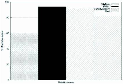
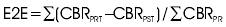
Figure 1 (a). Number of blind vehicles
Routing is one of the most important challenges in Vehicular Ad hoc Networks (VANETs). These networks involve a high cost in the real world experimentation. Thus, simulation is a useful alternative in conducting such a research. In this paper, two important routing protocols (AODV and DSDV) have been considered for testing in VANET environments. Performance evaluation has been accomplished for these two routing protocols using the CityMob mobility generator that generates the required urban mobility scenario files. Then, simulation has been done based on these scenario files using the NS-2 simulator. The performance of the routing protocols has been compared based on some routing metrics (Packet Delivery Ratio and End to End Delay) for different values for the speed of vehicles. The work has been done under Linux operating system.
The increasing demand of wireless communications and the needs of new wireless devices have led to worldwide research activities on autonomous, self-configuring, decentralized, and infrastructureless networks. Networks with such specifications are the basic philosophy behind Mobile Ad Hoc Networks (MANETs). The era of wireless communications began with the first successful demonstration of wireless information transmission by Nikola Tesla in 1893. However, it was not until the last decade of the twentieth centur y that wireless communications (e.g., cell phones) become ubiquitous [Bulent & Wendi, 2006].
In the recent years, rapid development in wireless communication networks has made Inter-Vehicular Communications (IVC) and Road-Vehicle Communications (RVC) possible in Mobile Ad Hoc Networks (MANETs). This has stimulated a new type of MANET known as the Vehicular Ad Hoc Network (VANET) [Radusch & Adrian, 2010]. VANETs are branch of MANETs but with distinguishing characteristics like, movement at high speeds, constrained mobility, sufficient storage, and processing power [Vivek, 2010]. The importance of VANETs has been recognized by many car manufacturers, governmental organizations, and the academic community. The Federal Communications Commission (FCC) has allocated spectrum for VANETs. Governments and some car manufacturers, such as Toyota, BMW, and Daimler-Chrysler have launched some important projects for VANET, such as Advanced Driver Assistance Systems (ADASE2), Crash Avoidance Matrices Partnership (CAMP), CARTALK 2000, Fleet Net, and CarNet [Bilal & Umar, 2010; Xi & Li, 2008].
Movement of vehicles on road will have constraints and limitations related to speed zones, traffic congestions, weather state, very high node mobility, limited freedom in mobility patterns, etc. These constraints may result in a group of clusters in network so that vehicles sometimes become unable to make direct connections (network discontinuity) between one node (in one cluster) to another (in other cluster) without assistance from other nodes. Available routing protocols for MANETs basically are not compatible with VANET scenario due to these limitations. Hence, simulation studies of these MANET routing protocols had been conducted to find whether they are appropriate or useable in VANETs [Shaikh, 2010; Lee, Lee, & Gerla, 2009].
Basically there are two types of routing protocols in MANETs; proactive and reactive routing protocols. Proactive MANET protocols (PMPs) periodically update routing information for each node. Thus, when a node wants to transmit at any given time, there will be available a fresh list of destinations and their routes by periodically distributing routing tables in the network. The main disadvantage of this approach is the amount of exchanged data for maintenance. Examples of this type are Destination Sequenced Distance Vector Routing (DSDV) and Cluster Head Gateway Switch Routing (CGSR). Reactive MANET Protocols (RMPs) do not maintain routes at any time. Instead of that, they will find routes when that is needed (on demand). In this type, nodes find routes by flooding network with Route Request packets. The main disadvantage here is the high time latency in finding routes. Also, excessive flooding can result in network clogging. Ad hoc On demand Distance Vector routing (AODV) and Dynamic Source Routing (DSR) are famous examples of reactive routing.
This paper aims to perform simulation and performance analysis of AODV and DSDV routing protocols using NS-2. This simulation will consider the specific environment of IVC. One can notice that most of the earlier research on analysis of routing protocols in VANETs has focused on either highway environment (in which the speed is high, little number of intersections exists, etc.) or in city environment (in which the speed is less, many number of intersections exist, etc.). Here, we will focus on Downtown environment (in which most congestions occur, vehicles can move only in low speeds most of the time, etc.) (Martinez & Cano, 2008;Fan & Narayanan, 2003; Andrea, Angelo, & Riccardo, 2010). Another goal is to more investigate the CityMob mobility model generator. This generator was designed by the Networking Research Group "Groupo de Redes de Computadores" (GRC) that belongs to the Technical University of Valencia (UPV). As far as the knowledge of the authors of this paper, there is only a little number of available researches based on using this generator due to the modernity of the generator [Martinez & Cano, 2008; Vossen, 2010]. Thus, we believe that one contribution of this paper is to shed more light on using CityMob in VANET research.
The remaining of this paper is organized as follows: Section 1 is a brief survey of some related works. Section 2 outlines the basic features of AODV and DSDV routing protocols. Some relevant simulation issues are explained in Section 3. Next, Section 4 is a description of our simulation environments. Then, our conducted performance analysis of the two routing protocols based on CityMob in VANET environment is presented in Section 5. Finally, the paper is concluded.
According to [Victor, Francisco, & Pedro, 2009], movement of vehicles can be described in the form of distinct clusters, which is also an observable scene. Therefore, in VANETs, routing protocols will be necessar y to make communication between these clusters. As discussed in Shaikh (2010), there are some routing protocols which are believed to be suitable from both of MANET and VANET perspectives. AODV and DSDV can be representative examples of such protocols. Shaikh's (2010) work considered these two protocols in city and highway density levels to evaluate the performance of Ad hoc routing protocol in realistic urban vehicular motion patterns so that it can be possible to make an improvement in providing Comfort Applications. In [Laiq, Nohman, & Aamir, 2009], a study was done to propose MANET anycast AODV routing protocol so as to make it adaptive for VANETs using VanetMobisim (a generator for vehicular mobility traces) under different metrics.
The work in [Surayati, Usop, & Abdullah, 2009] presented a study of some MANET routing protocols in grid environment. It made a comparison between AODV, DSDV, and DSR routing protocols, using performance metrics such as packet delivery fraction, average-end to end delay, and packet loss. In [Singla, Singla, & Kumar, 2009] performance evaluation of three routing protocols AODV, DSR, and DSDV was performed. The work addressed three main issues. The first was to find which routing protocol provides better performance in MANETs. The second issue was related to the factors that influence the performance of these routing protocols. Finally yet importantly, the major differences in these routing protocols under study were addressed. The research presented in [Josiane, Neeraj, & Guiling, 2009] was a design and implementation of two routing protocols; reactive protocol called RBVT-R and proactive routing protocol called RBVT-P. Then these two protocols were compared against representative protocols of MANETs (AODV, OLSR, and GPSR) and another representative protocol of VANETs (GSR). In [Vossen, 2010], a comparative study was done for scenario mobility generators according to software characteristics, maps type, mobility models, traffic models implemented, and trace formats support.
Ad hoc On Demand Distance Vector (AODV) is one of the most popular ad hoc routing protocols. Itenjoys a number of reviews which concluded that it could be the best for high mobility environment. AODV uses some features from DSR and some others from DSDV. It has monotonically increasing sequence numbers of the route entries of DSDV, and updates the route entries using a route discovery protocol [Wiberg, 2002]. When a node wants to transmit data to other node and the route to this node is unknown, it will broadcast Route Request packet (RREQ). This RREQ contains the last (fresh) sequence number for this route which assure for loop-free networks. Nodes which receive this RREQ packet update its routing table for source node address then this RREQ packet is broadcasted through the network until it reaches to specify destination node or to node have enough fresh route to destination. Each node that forwards the RREQ packet creates reverse route (backward pointer) to source node. The RREQ packet contains the address of the source node, broadcast identification, address of the destination, destination sequence number [Perkins & Royer, 2000].
When a node receives RREQ packet and the node is the destination or has route to destination, it firstly checks the sequence number of RREQ with the sequence number of route in its routing table which must be greater or equal to the RREQ sequence number. If the two sequence numbers are equal, it must check the hop count of route and select the smallest hop count then it generates the Route Reply (RREP) packet. If the received node is not the destination or has no route to destination, it will rebroadcast the RREQ packet to its neighboring nodes. The RREP packet is then sent to the source node with unicasting transmission. When the RREP is traversed through the route which was established by RREQ or the route from the destination, it will be updated the destination address.
On the other hand, Destination-Sequence Distance-Vector (DSDV) is a table driven routing protocol in which each node has a table of information. This table is updated periodically or when network change occurs [Shaikh, 2010]. So any change in the network will be broadcasted to every node of the network. The main contribution of the algorithm was to solve the Routing Loop problem. Every mobile station maintains a routing table that lists all available destinations, the number of hops to reach the destination, and the sequence number assigned by the destination node. The sequence number is used to distinguish stale routes from new ones and thus to avoid the formation of loops. The stations periodically transmit their routing tables to their immediate neighbors. A station also transmits its routing table if a significant change has occurred in its table from the last update sent. So the update is both time-driven and event-driven [Perkins & Bhagwat, 1994]. DSDV requires a regular update of its routing tables, which uses up battery power and a small amount of bandwidth even when the network is idle. Whenever the topology of the network changes, a new sequence number is necessary before the network reconverges. Thus, DSDV may not be suitable for highly dynamic networks [Surayati et al., 2009].
Simulation is usually used to model natural, machine or human systems in order to gain insight into their functioning. It is a very important mechanism to understand interactions between various systems, parts of which may be difficult to recreate or control in the real world. Hence, simulation is important tool in most research involving wireless networks, in which it is difficult to prepare wireless propagation environment, difficult to use real radio-wave based transmission, and non-trivial to use real wireless sensor/devices to present research ideas [Kavithea, 2009]. In network research area, we usually need to verify and validate multiple network computers and data links. Thus, the network simulator will be necessary to save a lot of money, time and allowing the network designers to test new networking protocols or change exiting ones in a controlled and reproducible manner.
As a comparison between real life and simulation research in MANETs, for example, nodes in real-life are powered by on-board batteries, equipped with sensors and navigation devices to do variety of applications from store-andforward to intelligent aggregation of data. In simulation, they are depicted with some of the above characteristics. Batteries may be depicted by a continuously decreasing numeric power indicator. Other things such as node architecture and OSI layers can also depicted efficiently with simulation. In simulation, nodes can execute protocol implementations and components of various layers, similar to their real time counterparts. Examples of such components are the wireless interface reception, propagation, noise, channel, etc. Other components include network devices (number of nodes, etc.), data traffic (levels such as TCP, etc.), and mobility scenarios. All these components can be represented in simulation in conventional ways [Kavithea, 2009].
There are many simulators such as Network Simulator 2 (NS- 2),OPNET Modeler, GloMoSim, and OMNeT++. But before going to select one of these simulators, there are some important issues to be determined, such as determining the specifications of simulation model so that the selected simulator must be general-purpose enough to provide the behavior of environment. Indeed, input/output data of the real system must be appropriate with the simulator and the design of experiment.
NS-2 is an open-source event-driven simulator designed specifically for research in computer communication networks. Since its inception in 1989, NS-2 has continuously gained interest from industry, academia, and government. Having been under constant investigation and enhancement for years, NS-2 now contains modules for numerous network components such as routing, transport layer protocols, applications, etc. NS-2 has become the most widely used open source network simulator, and one of the most widely used network simulators [Issariyakul & Hossain, 2009]. NS-2 can be applied on very large number of applications, protocols, network types, network elements and traffic models. All these in NS-2 are called "simulated objects". Hence, we have chosen NS-2 as the simulation tool for this work because NS-2 efficiently supports networking research and education. Also, Ns-2 is suitable for designing new protocols, comparing different protocols, and for traffic evaluations [Martinez & Toh, 2009; Altman & Jimenez, 2004].
CityMob is one of the relatively recent scenario generators that can be used to generate scenario files as one input to the NS-2 simulator. CityMob generator is easy to install and easy to use. The CityMob user interface shows speeds as km/h, in which the nodes are named with a string followed by a number from 0 to N-1. Indeed, CityMob has the following capabilities: Multiple lanes in both directions for each street, vehicle queues belong to traffic density, and may have more than one downtown [Vossen, 2010]. Compared to other scenario generators, CityMob has the shortest warning notifications. CityMob also has a minimum of blind vehicles, and thus the number of packets received will be maximized, as illustrated in Figure 1 [Martinez & Toh, 2009]. It is obvious that using different VANET generators, different performance results will be obtained.
Figure 1 (a). Number of blind vehicles
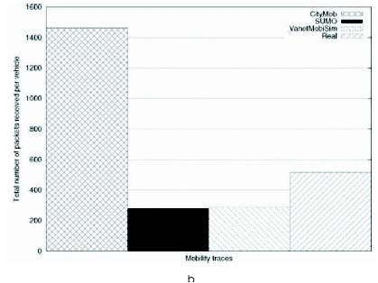
Figure 1(b). Total number of received packets for different scenario generators [Vivek,2010]
The traffic model generator will be applied to determine the traffic source, maximum connections between nodes, and the rate of transformation. The traffic model can be selected as Constant Bit Rate (CBR), where the packet size will be chosen as 512. CBR is a network communication model and there is another model called Variable Bit Rate (VBR). These models are basic to define wireless communication among mobile nodes such as to enable simulating the various routing protocols. The main idea is to randomly select node pairs as sources and destinations. The traffic generator is embedded within NS-2 [Chung & Claypool, 2002].
The simulation environment used in this work is under Linux (Ubunto 9.04) operating system. The simulator tool used is NS-2 (version 2.34) [more details on this simulator can found at www.isi.edu/nsnam/ns/]. The mobility model used is the Downtown mobility model that mathematically constrains the movement in down town area. The CityMob Version 2 is the generator used to generate scenario files based on this movement. After these information applied to NS-2, the resultant (tracefile.tr) will contain all information in thousands of lines. Hence, there is a need to analysis theses information. The tool used for this is called AWK (after Alfred Aho, Peter Weinberger, and Brian Kernighan), which reads raw data line by line. After this analysis, results are drawn using GNUplot. Figure 2 shows a general view of the used simulation environment. More detailed illustration of the simulation environment is depicted in Figure 3. This figure shows the type of scenarios files, traffic file generator, two output files from NS-2, and the drawing tool.
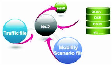
Figure 2. General view of the Simulation Environment
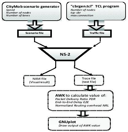
Figure 3. Details of the Simulation Environment and tools used for Analysis and Plotting in Linux
Simulation parameters are summarized in Table I. The authors applied CBR sources (for traffic model) that started at different times to get a general view of how routing protocols behave.
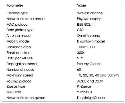
Table I. Simulation Parameters Of Speed Scenarios
In Downtown Model, traffic is not uniformly distributed. Instead of that, there are zones in higher density and low speed usually in downtown. But in outskirts, vehicles are of less density and higher speeds. The area of downtown can be determined by coordinates (start-x, end-x, start-y, and end-y) and must never cover more than 90%. Figure 4 shows the downtown area that includes the dark buildings. The darker rectangles represent vehicles, the shadowed rectangles represent vehicles stopped at semaphores, and crosses represent damaged cars sending warning packets (Martinez & Cano, 2008).
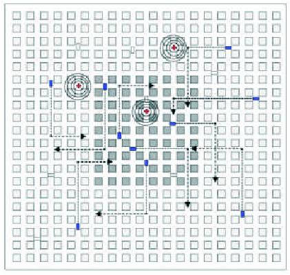
Figure 4. Example of the downtown model
The DownTown Route System can be formally introduces as follows:

Where RD represents DownTown Route System, BD is the bundle set and the RD represents set of DownTown routes. There are different kinds of bundles such as Starts-bundles, End-bundles, Transit-bundles, Cross-bundles and so on. Each one of these bundles is mathematically constrained by some formulas. For example for the Start-bundle, the following equations determine the movements of one vehicle in horizontal blocks:
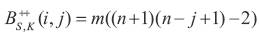
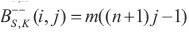
where represent Starting-bundle into horizontal blocks, m represent the length of street (number of cells forming the street), n enumerate horizontal streets by an increasing even index {0,2,...,n}, starting from the left-top corner and (i, j) pair of coordinates to determine the crossway. It is possible to compute Starting-bundles in vertical blocks simply by replacing index j with i. All mathematical constraints of other bundles for this mobility model can be found in [Andrea et al., 2010]. The signs (++,--,+-, and -+) mean that there are four possibilities to one vehicle; still in the same route, take left side, take right side, and go back.
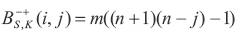
User can determine followings: total number of nodes, simulation time, map size, maximum speed, distance between consecutive streets, and number of damaged nodes. CityMob user interface show speeds as km/h. Simple and Manhattan mobility models have similar behavior but Manhattan has quick packet propagation. Downtown model shows the best results on realism and flooding behavior. It allows information quickly disseminated in network, as shown in Figure 5 (Bilal & Umar, 2010).
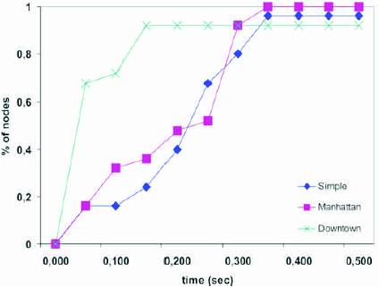
Figure 5. Comparison among three mobility models in quick information disseminating
Streets in Downtown Mobility Model are arranged as the Manhattan style grid with uniform block size on simulation area. These streets have two ways, with lanes in both directions. Car movements are constrained by these lanes. Speed of vehicles will be randomly constrained to user defined range of values. Semaphores are simulated in this model in different locations (not only at intersections) with variant delays. Downtown model adds traffic density on special ways similar to real town, which means that traffic is not uniformly distributed. Hence, in this model there are areas with higher density of vehicles. These zones often are in downtown and the velocity of vehicles must be slow comparing with outskirts.
There are several metrics to evaluate routing protocols. Performance metrics are important to measure the performance and activities that are running in NS-2 simulation so as to enable the choice of the best routing protocol according to the performance results. The two metrics used in this research are:
The packet delivery ratio in this simulation is defined as the ratio between the number of packets sent by constant bit rate (CBR) sources (in application layer) and the number of received packets by the CBR sink at destination, as follows [Surayati et al., 2009]:

where PDR is Packet Delivery Ratio, "CBRPR by CBRsinks " is CBR Packets Received by CBR Sinks,and "CBRPS by CBRSources " is CBR Packets Sent by CBR Sources. The above equation describes percentage of the packets which reaches the destination.
There are some delays that happen in packet transition to receiver. This is mainly caused by buffering during route discovery latency, queuing at the interface queue, retransmission delays at MAC layer, and the propagation and transfer times. For each received packet, the average of End-to-End delay will be the time difference between every CBR packet sent and received divided by the total time difference of CBR packets. The lower the average end-to-end delay is the better application performance [Gillani, 2007]:
Where E2E is End to End delay, CBRPRT is the time of CBR Packets Received by CBR Sinks.CBRPST is the time of Packets Sent by CBR Sources, and CBRPR is only for the packet that had been received.
In this simulation, speed scenarios of five different speeds (10, 20, 30, 40 and 50 km/h) have been taken with constant numbers of vehicles. The performance comparisons have been made between AODV and DSDV protocols based on the two network important metrics PDR and E2E for each one of these scenarios files. In each scenario, identical mobility model and traffic scenario have been used. Hence we assume POI: (300.0,400.0; 600.0,700.0). The probability of vehicle to visit POI has been assumed to be 0.5. That means each vehicle has 50% probability to enter the area of POI.
In these scenario files, we have chosen the simulation of 60 nodes in 1000X1000 square meters area. Other simulation environment parameters are illustrated in Table I.
Simulation results for the effect of speed change on E2E are shown in Figure 6. From this figure, we can notice that the E2E delay in DSDV is lower than AODV. Topology changes affect all types of routing protocols but they are much more significant for routing protocols which do not have good technique in updating and storing structure in routing table. This is because all nodes which construct the network will need to send more packets to know the effects of new topology in periodical way. Hence, the E2E delay will be low at first (low speed) and after the speed increases to 40km/h the delay will increase. On the other hand, AODV has high delay and that because AODV is a reactive routing protocol. So, almost every time there is a need to access to a specific destination, there will be a search in network (if there is no route in the node routing table). This introduces a delay. However, as AODV does not highly effected by the change of topology (due to the high speed), when the speed exceeds about 60km/h, we can notice that the delay in AODV is become closer from DSDV a proactive one, while DSDV E2E delay is increasing as vehicles mobility increasing. The good behavior of AODV routing protocol in speed of 60 km/h belong to the increase of the packet delivery of the network on this speed by reducing the buffering time of these packets.
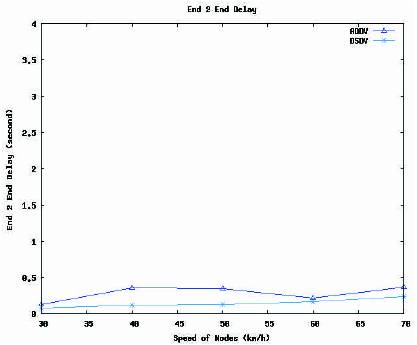
Figure 6. Effect of change in vehicle speeds (km/h) on E2E delay
Note that the speed in downtown area is limited from 5-30 km/h for all time of simulation. Thus, the performance of routing protocols will be affected by this area. This is due to the foundation mathematics of the Downtown mobility model which governs this area. However, if there is a need to simulate other speeds in different circumstances, we must consider another mobility model such as Manhattan mobility model, City Section mobility model, and Free mobility model [Marco et al., 2007].
PDR is the relation between the application layer source packets sent by one vehicle to the number of received packets by sinks in the destination vehicle. From this ratio, we can see the lost packets by transportation layer and their effect on maximum throughput of the network can support. Simulation results for the effect of speed change on PDR are illustrated in Figure 7. From this figure, we can see AODV generally has good PDR values. When the speed of vehicles increases, the PDR decreases in DSDV more than AODV because of the increasing change of topology due to movement of vehicles. In high mobility environments, topology changes rapidly and AODV can adapt to the changes quickly since it only maintains one route that is actively used. Form the results; we can see that AODV starts with approximately in 0.91 and still around that until the final reading at approximately in 0.89. DSDV starts at approximately in 0.71 and after that we have large amount of PDR decrease before reaching to a final reading of 0.62 approximately. Thus, AODV generally outperforms DSDV in PDR.
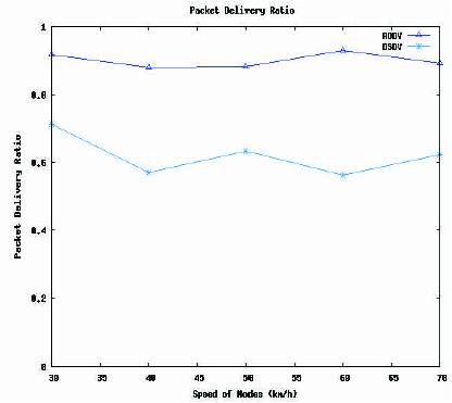
Figure 7. Effect of change in vehicle speeds (km/h) on PDR
In this work, the authors have performed simulation and comparison study between two routing protocols (AODV and DSDV) using CBR traffic. This comparison has been accomplished based on two important metrics; packet delivery ratio and end to end delay with respect to the change in speed of nodes. This is because the speed is very important factor in VANETs. The results in general show better performance of AODV compared to DSDV in VANET environment in term of the packet delivery ratio. High mobility results in frequent link failures and the overhead involved in updating all the vehicles with the new routing information as in DSDV is much more than that involved AODV, where the routes are only created when required (on-demand). This reduces the DSDV efficiency in high mobility.
For end to end delay, DSDV has been better than AODV. Whereas DSDV uses the proactive table-driven routing strategy while AODV use the reactive On-demand routing strategy. The updating process in DSDV is both time-driven and event-driven which reduces the required time for new changes in mobility. From above discussions we can conclude that for applications which need high packet delivery, it is recommended to use AODV routing protocol. While for applications which need low E2E delay without care to packet delivery, we can better use DSDV.
For future work, we are planning to simulate different routing protocols on this environment and analyze their performance. This can help people to select the appropriate routing protocol for each particular case. Also, performing simulation based on other mobility models will be considered. In addition, the good behavior of AODV in PDR issue is pushing us to do further research in order to enhance this routing protocol in E2E metric terms for VANET applications.