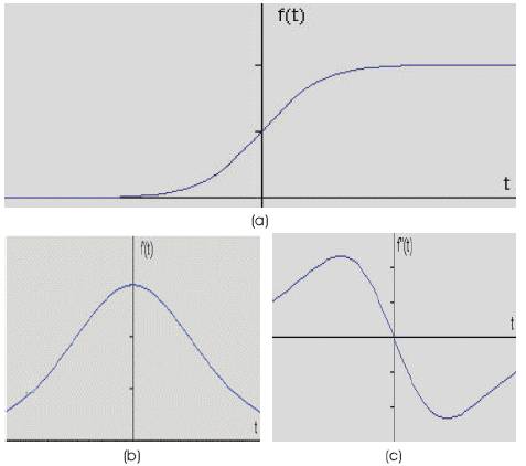
Figure 1. (a) Gray level profile of an image. (b) First order derivative of the profile. (c) Second order derivative of the profile.
Medical images are diagnosed and demonstrated with their regional structures. Edge detection is a fundamental element in the field of image processing and computer vision for the extraction of features. Edge detection identifies and captures sharp intensity changes in an image. Medical image edge detection focus on object recognition of human organs. To detect the severity of disease several medical approaches like CT, MRI, PET, US and DICOM can be used. In this paper performance of CT and DICOM images using morphology and edge detection algorithms are evaluated in noisy environment. A comparision of different edge detecting algorithms by using several noises is performed and evaluated based on correlation coefficient and PSNR. The outcomes evaluate the resistivity of operators in presence of noise.
An image is defined as a two dimensional light intensity function f(x,y),where x and y are spatial coordinates, and the value f at any pair of coordinates (x,y) is called intensity or grey level value of the image at that point. Edge detection is one of the most commonly used operations in image analysis. An edge is defined by a discontinuity in grey level values. Edge can also be defined as the boundary between an object and the background. Edges are the sign of lack of continuity, and ending. As a result of this transformation, edge image is obtained without encountering any changes in physical qualities of the main image. Edge detection reduces the amount of data that is to be processed without disturbing the structural properties of the image. Edge detection filter mainly improves the appearances of the blurred images. Edge detection converts original image into edge image by forming boundaries or outlines. The shape of the edges in images depends on many parameters: the geometrical and optical properties of the object, the illumination conditions, and the noise level in the image [1]. Medical image detection is a line through which the work of object recognition of the human organs such as lungs, brain and ribs, abdominal extremities and it is an essential pre- processing step done in medical image segmentation. In real world applications, medical images contain object boundaries and object shadows and noise [2]. This paper distinguishes the exact edge from noise and which operator better suits for the noise environment to extract the edges.
In the past two decades several algorithms were developed to extract the contour of homogenous regions within a digital image. Edge detection being a crucial part a lot of interest and attention is focussed on most of the algorithms. L.J. Spreeuwers and F. vander Heijden [3] evaluated the performance of edge detectors using average risk with arbitrary test images which estimates the probabilities on different types of errors. Mike Heath et al. [4]has made comparison of four edge detectors which allows to make quantitative comparisons using subjective ratings made by people using experimental procedure and statistical methods borrowed from psychology. Tuba Sirin et al. [5] made evaluation of competitive learning algorithms for edge detection enhancement (segmentation) followed by an edge detector and concluded that the performance of two stage algorithm is superior to one stage algorithm. Shin M.C et al [6] presented an evaluation of edge detector performance using structure from motion task and concluded that canny detector had the best test performance. Mohesen Sharifi et al. [7] introduces a new classification of most important and commonly used edge detection methods namely ISEF, Canny, Marr-Hildreth, Sobel, Kirsch and Lapalcian. Raman Maini and J.S.Sohal [8] evaluated the performance of Prewitt edge detector for noisy images and concluded that Prewitt operator works quite well for images corrupted with Poisson noise. M.Roushdy [9] made a classified and comparative study of edge detection algorithms using morphological filter.
Segmentation procedures partitioning an image into its constituent parts or objects. In general, the more accurate the segmentation, the more likely recognition succeeds. The concept of segmenting an image based on discontinuity and similarity. segmentation refers to the process of partitioning a digital image into multiple segments (sets of pixels, also known as super pixels). The goal of segmentation is to simplify and/or change the representation of an image into something that is more meaningful and easier to analyze. Image segmentation is typically used to locate objects and boundaries (lines, curves, etc.) in images. The result of image segmentation is a set of segments that collectively cover the entire image, or a set of contours extracted from the image.
Figure 1. (a) Gray level profile of an image. (b) First order derivative of the profile. (c) Second order derivative of the profile.
The major edge detecting methods may be grouped into two categories, Gradient and Laplacian. The gradient method detects the edges by looking for the maximum and minimum in the first derivative of the image. The Laplacian method searches for zero crossings in the second derivative of the image to find edges[7].
Gradient edge detectors: It includes algorithms such as: Sobel (1970), Prewitt (1970), Kirsch (1971), Robinson (1977), Frei-Chen (1977), Deatsch and Fram (1978), Nevatiaandbabu (1980), Ikonomopoulos (1982), Davies (1986),Kitchen and Malin (1989), HancockandKittler (1990), Woodhalland Linquist (1998), and Young-won and Udpa (1999)[1,10,11,13].
It is a simple, quick to compute, 2-D spatial gradient measurement on an image. It highlights regions of high spatial frequency which often correspond to edges.
One kernel is simply the other rotated by 90°. This is very similar to the Sobel operator. The gradient magnitude is given by:
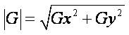
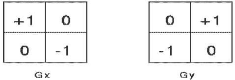
Figure 2. Roberts cross kernels
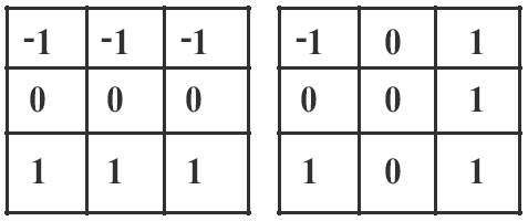
Figure 3. Sobel operator masks
A way to avoid gradient calculation about an interpolated point between pixels is to use a 3 x 3 neighbourhood for the gradient calculations. The Sobel operator is the magnitude of the gradient computed by:
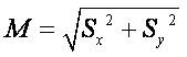
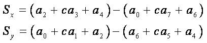
Sx and Sy can be implemented using the masks with constant c=2
The Prewitt operator uses the same equations as the Sobel operator, except that the constant c= 1.Therefore:
Unlike the Sobel operator, this operator does not place any emphasis on pixels that are closer to the centre of the masks.
Another approach is to apply rotated versions of these around a neighbourhood and “search” for edges of different orientations; there are eight kirsch kernels which can run on the image to get edges in different directions. By rotating the above mask by clock wise by eight times edges in different directions are obtained.
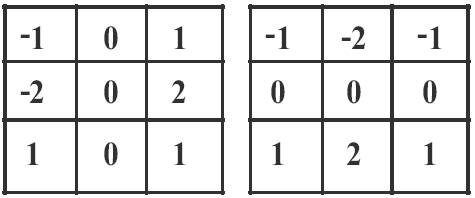
Figure 4. Prewitt operator masks
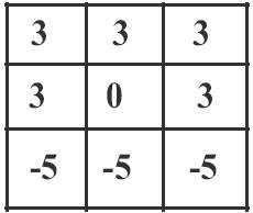
Figure 5. Kirsch compass kernels
The aim of Canny edge detection was to develop an algorithm that is optimal which runs in 5 steps:
This uses second derivative [12] and includes laplacian operator and second directional derivative.
This was invented by Marr and Hildreth (1980) who combined Gaussian filtering with the Laplacian. This algorithm is not used frequently in machine vision. Those who continued his way were Berzins (1984), Shoh, sood and Jain (1986), Huertas and Medioni (1986) [12, 11]. The second derivative profile can be obtained by using the masks shown in Figure 6(a, b), the gradient obtained to original image is illustrated in Figure 7(a, b).
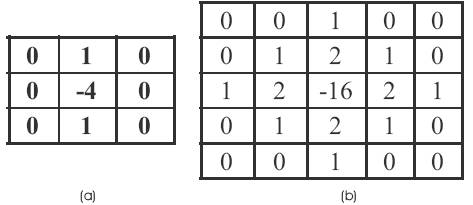
Figure 6. (a) 3x3 Laplacian mask. (b) 5x5 Laplacian mask.
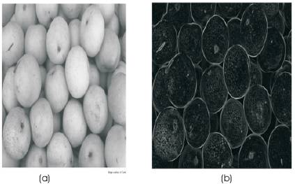
Figure 7. (a) original image. (b) gradient of the image.
It is always important to choose edge detectors that fit best to the application. In this respect some advantages and disadvantages of algorithms within the context of our classification are.
The Sobel and Prewitt operators are very simple to detect their edges and orientations. LoG uses second derivative, finds exact location of edges and tests wider area around the pixel. Gaussian edge detector like Canny uses probability for finding error rate. They have better detection and reduce noise by smoothing the image.
First derivative operators have inaccurate detection sensitivity in the presence of noise. The LOG cannot find edge orientation as it uses Laplacian filter and cannot respond correctly at corners where the intensity function varies. Canny edge detectors include complex computations and are time consuming.
It is introduced in 1972. It is also called as Computer Axial Tomography (CAT) or X-Ray computer tomography. It is used for medical & industrial imaging and used to diagnose head, lung, pulmonary angiogram, cardiac, abdominal extremities. Image quality is a 8-bit pattern.
CT data increases radiologist efficiency and provides more accurate diagnosis for lung cancer. Eliminates superimposition of images of structures. High contrast resolution.
Uses high level of ionising radiation that alters DNA of each cell of the body. Inferior soft tissue contrast compared to DICOM.
DICOM stands for Digital Imaging and Communications in Medicine and represents universal and fundamental standard in digital medical imaging. It is not just a image or file format. It provides all necessary tools for diagnostically accurate representation and processing of medical imaging data. It is an all-encompassing data transfer, storage, and display protocol & has high diagnostic standards and best performance. DICOM provides much of the ease and flexibility in work. DICOM-based workflow builds a robust and efficient radiology practice. DICOM is used to collect the original medical images. DICOM can send, distribute an store images irrespective of machine, manufacturer or modality. DICOM controls proper image display and image post processing.
A universal standard of digital medicine. Excellent Image quality - supports up to 65,536(16 bits) shades of gray for monochrome image display. Full support for numerous image. Complete encoding of medical data.
Morphology refers to the study of shapes and structures. These operators transform the original image into another image through the iteration with other image of a certain shape and size which is known as structuring element. The basic morphological filters are opening and closing with structuring elements. The binary morphology can be easily extended to gray-scale morphology [18]. Morphological image analysis can be used to perform Object extraction Image filtering operations, such as removal of small objects or noise from an image segmentation operation. Morphological image analysis can be used to perform image filtering, image segmentation, and measurement operations. Mathematical morphology theory must been changed into set. Mathematical morphology uses structuring element, which is characteristic of certain structure and feature, to measure the shape of image and then carry out image processing. Based on set theory, mathematical morphology is the operation which transforms from one set to another. Morphological edge detection algorithm selects appropriate structuring element of the processed image and makes use of the basic theory of morphology including erosion, dilation, opening and closing operation. The medical modalities CT and DICOM described above are shown in Figure 8(a, b), the morphological filter operations are clearly visualised in Figure 9(a, b).
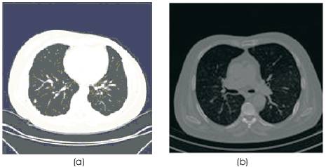
Figure 8. (a) CT image (b) DICOM image
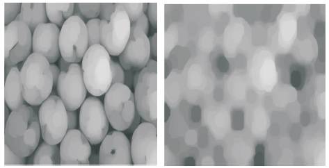
Figure 9. (a) open operation (b) open & close operation
Noise is considered to be any measurement that is not a part of the phenomena of interest. Images are prone to different types of noises Such as Gaussian, speckle, salt & pepper and Poisson noise. The image data dependency arises because detection and recording processes involve random electron emission having a Poisson distribution with mean response value [14]. Gaussian noise that occurs in all recorded images to a certain extent is detector noise. This kind of noise is due to the discrete nature of radiation. The noise has zero-mean Gaussian distribution described by its standard deviation or variance [15]. Another noise is data drop out noise commonly referred as speckle noise. This noise is, in fact caused by errors in data transmissions [16]. The corrupted pixels are either set to the maximum value, which is something like a snow in image. The type of noise caused by errors in data transmission. single pixels are set alternatively to zero or to the maximum value giving the image a salt and pepper like appearance [17].
The Performance of edge detecting operators is evaluated for CT & DICOM lung images with and without noise. The methods considered are Sobel, Prewitt, Roberts, Canny, LOG, Kirsch, and Morphological. The noise added is Gaussian, speckle, salt & pepper and Poisson noise.
The edge images of the operators are computed in MATLAB applied to CT & DICOM Lung image. These images are shown in Figures 10 & 11(a, b, c, d, e, f & g) and are compared with the same operators applied to CT & DICOM Lung image after adding noise.
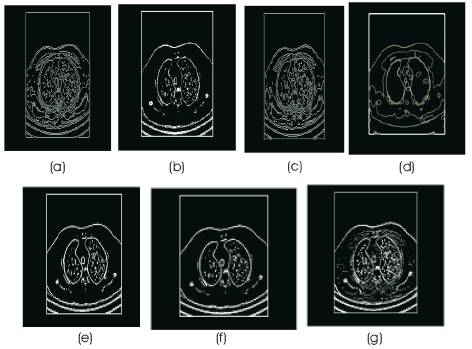
Figure 10. Edges on CT lung image without noise using (a) canny (b) kirsch (c) LoG (d) morphological (e) sobel (f) prewitt and (g) roberts edge operators
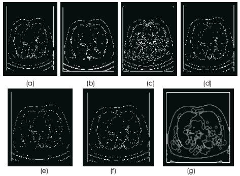
Figure 11. Edges on DICOM lung image without noise using (a) Canny (b) Kirsch (c) LoG (d) Prewitt (e) Roberts (f) Sobel (g) Morphological
Noises are added to CT & DICOM Lung image with default value and Gaussian noise with zero mean and standard deviation values σN= 5, 11, 25.
The results of various methods on noise added CT lung image are shown in Figures 12,13,14,15,16,17 & 18(a, b, c, d). CT & for DICOM lung Figures 19,20,21,22,23,24& 25(a, b, c, d).
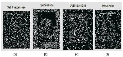
Figure 12. Canny operator on CT image with noises (a) Salt & Pepper (b) Speckle (c) Gaussian and (d) Poisson noise
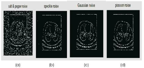
Figure 13. Sobel operator on CT image with noises (a) Salt & pepper (b) Speckle (c) Gaussian and (d) Poisson noise
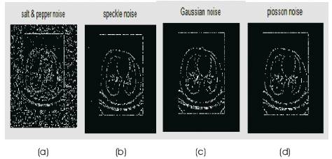
Figure 14. Prewitt operator on CT image with noises (a) Salt & pepper (b) Speckle (c) Gaussian and (d) Poisson noise
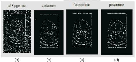
Figure 15. Roberts operator on CT image with noises (a) Salt & pepper (b) Speckle (c) Gaussian and (d) Poisson noise
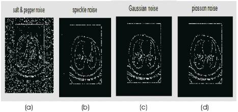
Figure 16. kirsch operator on CT image with noises (a) Salt & pepper (b) Speckle (c) Gaussian and (d) Poisson noise
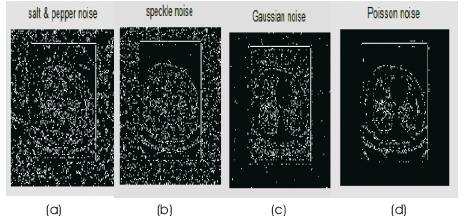
Figure 17. LoG operator on CT image with noises (a) Salt & pepper (b) Speckle (c) Gaussian and (d) Poisson noise
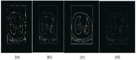
Figure 18. Morphological operator on CT image with noises (a) Salt & pepper (b) Speckle (c) Gaussian and (d) Poisson noise
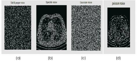
Figure 19. Canny operator on DICOM image with noises (a) Salt & pepper (b) Speckle (c) Gaussian and (d) Poisson noise
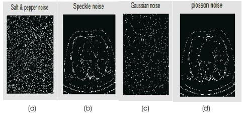
Figure 20. Sobel operator on DICOM image with noises (a) Salt & pepper (b) Speckle (c) Gaussian and (d) Poisson noise
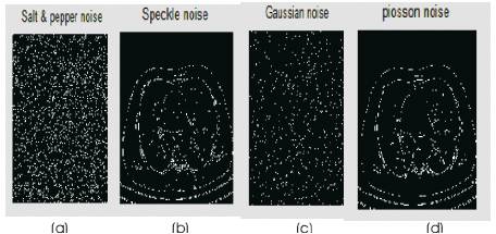
Figure 21. Roberts operator on DICOM image with noises (a) Salt & pepper (b) Speckle (c) Gaussian and (d) Poisson noise
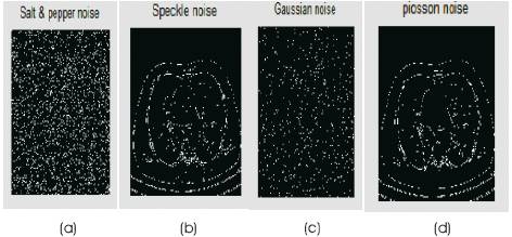
Figure 22. Prewitt operator on DICOM image with noises (a) Salt & pepper (b) Speckle (c) Gaussian and (d) Poisson noise
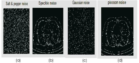
Figure 23. Kirsch operator on DICOM image with noises (a) Salt & pepper (b) Speckle (c) Gaussian and (d) Poisson noise
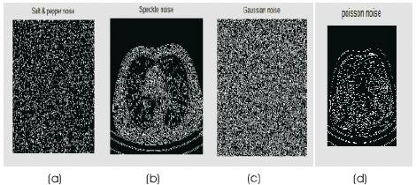
Figure 24. LoG operator on DICOM image with noises (a) Salt & pepper (b) Speckle (c) Gaussian and (d) Poisson noise
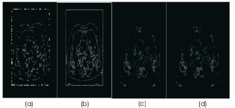
Figure 25. Morphological operator on DICOM image with noises (a) Salt & pepper (b) Speckle (c) Gaussian and (d) Poisson noise
The parameters used to evaluate the performance of different methods is correlation coefficient, which defines the closeness of the edge images of different methods in the noisy environment to the original edge images without noise and SNR, estimates degradation introduced with noise addition. As the value of sigma increases the Gaussian filter also increases and this implies more blurring, required for noise images for detecting large edges. The larger the scale of Gaussian the localisation of the edge becomes less accurate. Smaller values of sigma implies smaller Gaussian filter which limits the amount of blurring, maintaining finer edges in the image. The user can choose the algorithm by adjusting these parameters to adopt in different environments. The values for correlation coefficient and SNR are shown in Tables 1 & 3 for CT lung and in Tables 5 & 6 for DICOM lung with Gaussian & Poisson noises. Tables 2 & 4 represent correlation coefficient and SNR for CT & DICOM with salt & pepper and speckle noise.
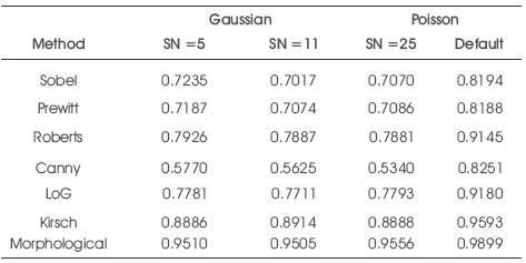
Table 1. Correlation coefficient for CT lung with Gaussian and Poisson noise
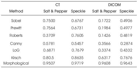
Table 2. Correlation coefficient for CT & DICOM lung with salt & pepper and speckle noise
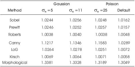
Table 3. SNR for CT lung with Gaussian and Poisson noise
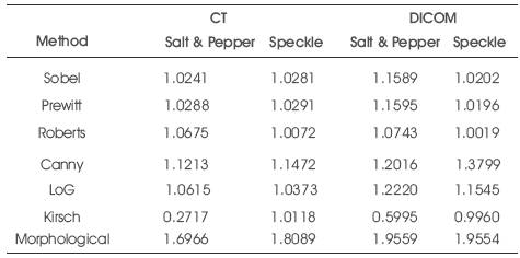
Table 4.SNR for CT & DICOM lung with salt & pepper and speckle noise
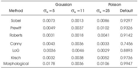
Table 5.Correlation coefficient for DICOM lung with Gaussian and Poisson noise
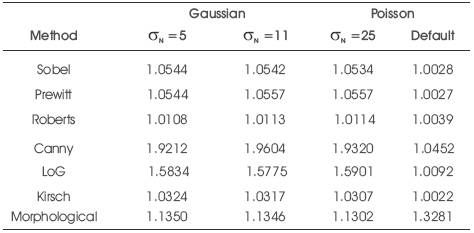
Table 6. SNR for DICOM lung with Gaussian and Poisson noise
Among all the operators such as sobel, prewitt, Roberts, Canny edge detection algorithm is computationally more expensive. However the canny edge detection algorithm performs better than all these operators almost in all the scenarios. Evaluation of images under noise conditions shows that canny, LoG, sobel, prewitt, Roberts exhibits better performance respectively.
Edge detection is the initial step in object recognition, it is essential to know the differences between edge detection methods.
In this paper the evaluation of different edge detecting methods is performed on CT & DICOM medical images. Four types of noises are Gaussian, salt & pepper, speckle and Poisson. From visual examination of the results, it can be noticed that Morphological operator exhibits superior performance than all the edge operators and well resist to noise. LOG, Canny methods exhibit better performances in noisy conditions and partially resistant to noise. When the content in the image has simple structure it has a non uniform contrast. Sobel and Prewitt performances are almost similar for all noises. Kirsch operator exhibits better performance than Sobel and Prewitt. The detected edges in the noise conditions decreases when compared with the edge images of the methods without noise. Signal to Noise ratio decreases as noise increases. Canny operator shows better performance compared to all other methods but is inferior to Morphological.
This work can be further extended in future with all these noises by developing a new or improved method using the existing software tools and make the segmentation process easier and flexible for any type of modality.