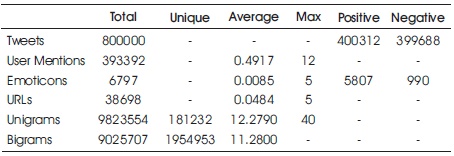
Table 1. Statistics of Pre-processed Train Dataset (Joshi & Deshpande, 2018)
To perform sentiment analysis, a number of machine learning and deep learning approaches were utilised in this paper to address the challenge of sentiment categorization on the Twitter dataset. Finally, on the Kaggle's public leaderboard, a majority vote ensemble approach has been used using 5 of our best models to get a classification accuracy of 83.58 percent. Various strategies for analysing sentiment in tweets (a binary classification problem) have been compared. The training dataset should be a CSV file with the following columns: tweet_id, sentiment, tweet, where tweet_id is a unique integer identifying the tweet, sentiment is either 1 (positive) or 0 (negative), and tweet is the tweet enclosed within "". For library requirements particular to some methods, such as Keras with TensorFlow backend for Logistic Regression, MLP, RNN (LSTM), and CNN for XGBoost, we used the Anaconda Python distribution. Preprocessing, baselines, Naive Bayes, Maximum Entropy, Decision Trees, Random Forests, Multi-Layer Perception, and other techniques that are implemented.
Sentiment analysis on Twitter refers to the use of advanced text mining algorithms to study the sentiment of a text (in this case, a tweet) in terms of positive, negative, and neutral. It is also known as Opinion Mining, and it is used to analyse conversations, opinions, and sharing of ideas (all within the context of tweets) in order to determine commercial strategy, political analysis, and public policy. Sentiment analysis is frequently used to uncover trends in tweet content, which are then examined using machine learning algorithms. Sentiment analysis is an important tool in the field of social media marketing because it will be discussed on how it can be used to forecast personal behaviour of an online user. Sentiment analysis is used to investigate the sentiment of a certain post or a specific topic.
Text comprehension could be a significant issue to resolve. One method could be to rank the relevance of phrases within the text and then create a summary of the content based on the important numbers. These systems rely on machine learning approaches like classification rather than manually generated rules. Classification is an automatic system that must be fed sample text before providing a category, such as positive, negative, or neutral. It is used for sentiment analysis. Urgent concerns will inevitably develop, and they must be dealt with as soon as possible. A Twitter complaint, for example, might easily turn into a public relations catastrophe if it goes viral. While it may be tough for your team to predict a crisis before it occurs, machine learning algorithms can easily detect these circumstances in real time.
The frequency distribution of various components of speech (either independently or in combination with other parts of speech) throughout a specific class of labelled tweets is commonly used to derive patterns. Twitter-based features are more casual and relate to how people express themselves on online social networks and condense their feelings into the limited 140-character space provided by Twitter.
Twitter hashtags, retweets, word capitalization, word lengthening, question marks, URL presence in tweets, exclamation marks, internet emoticons, and internet shorthand/slangs are just a few examples.
Sentiment analysis within the domain of micro-blogging could be a relatively new research topic so there's still plenty of room for further research in this area. A decent amount of related prior work has been done on sentiment analysis of user reviews, web blogs/articles, and phraselevel sentiment analysis. They differ from Twitter, mainly due to the 140 character limit per tweet, which forces the user to express their opinion in a very short text (Boguslavsky, 2017; Dos Santos & Gatti, 2014; TextBlob, 2017). The simplest results were reached in sentiment classification using supervised learning techniques like Naive Bayes and Support Vector Machines, but the manual labeling required for the supervised approach is incredibly expensive (Poria et al., 2015). Some work has been done on unsupervised and semi-supervised approaches, and there is a lot of room for improvement (Kiritchenko et al., 2014).
Various researchers are testing new classification features and techniques. They often compare their results to baseline performance. There is a desire to correct and formal comparisons between these results are made by different features and classification techniques to select the most effective for specific applications. This is a really simplistic assumption but it appears to perform fairly well. To use unigrams as features, align them with a specific preset polarity and take the average general polarity of the text, where it is the final polarity of the text (Duh et al., 2015; Statista, 2019). It is easy to figure out by adding the preceding poles of individual unigrams. The previous polarity of the term will be positive if the word is usually associated with good connotations, such as "sweet," and negative if the word is mostly associated with negative connotations, such as "evil" over there. Within the model, there can even be degrees of polarity, implying what proportion is indicative of it: A word for that specific group of people (Alm, 2011; Jiang et al., 2011). The word "wonderful" is a strong one. Subjective polarity and positivity go hand in hand, but "decent" may have positive a prior polarity but poor subjectivity.
Twitter is a popular social networking website where members create and interact with messages known as “tweets”. This serves as a means for individuals to express their thoughts or feelings about different subjects. Various different parties such as consumers and marketers have done sentiment analysis on such tweets to gather insights into products or to conduct market analysis. Furthermore, with the recent advancements in machine learning algorithms, it has been able to improve the accuracy of our sentiment analysis predictions. In this report, an attempt has been made to conduct sentiment analysis on “tweets” using various different machine learning algorithms. Also, many researches (Gokulakrishnan et al., 2012; Kouloumpis et al., 2011; Saif et al., 2012) attempted to classify the polarity of the tweet where it is either positive or negative. If the tweet has both positive and negative elements, the more dominant sentiment should be picked as the final label.
The dataset from Kaggle has been crawled and labeled positive/negative is used for the study. The data provided comes with emoticons, usernames and hashtags which are required to be processed and converted into a standard form. There is also a need to extract useful features from the text such as unigrams and bigrams which is a form of representation of the “tweet”.
Various machine learning algorithms have been used to conduct sentiment analysis from the extracted features. However, just relying on individual models did not give a high accuracy, so the top few models have been picked to generate a model ensemble. Ensemble is a form of metalearning algorithm technique where different classifiers have been combined in order to improve the prediction accuracy. Finally, the experimental results and findings are reported.
The information is provided in the form of commaseparated values (CSV) files including tweets and their associated feelings. The training dataset is a CSV file with the following columns: tweet_id, sentiment, tweet, where the tweet_id is unique, emoticons help predict sentiment, but URLs and references to persons do not. As a result, URLs and references can be disregarded. There are also misspelt words, excessive punctuation, and words with a lot of repeated letters within the words. As a result, the tweets must be pre-processed in order to normalise the dataset.
The provided training and test dataset have 800000 and 200000 tweets respectively. Preliminary statistical analysis of the contents of datasets, after pre-processing as described is shown in Tables 1 and 2.
Table 1. Statistics of Pre-processed Train Dataset (Joshi & Deshpande, 2018)
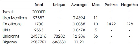
Table 2. Statistics of Pre-processed Test Dataset (Joshi & Deshpande, 2018)
Raw tweets scraped from Twitter generally result in a noisy dataset. This is due to the casual nature of people's usage of social media. Tweets have certain special characteristics such as re- tweets, emoticons, user mentions, etc. which have to be suitably extracted. Therefore, raw Twitter data has to be normalized to create a dataset which can be easily learned by various classifiers. We have applied an extensive number of pre-processing steps to standardize the dataset and reduce its size. We first do some general pre-processing on tweets as suggested by Joshi and Deshpande (2018):
Users often share hyperlinks to other webpages in their tweets. Any particular URL is not important for text classification as it would lead to very sparse features. Therefore, we replace all the URLs in tweets with the word URL. The regular expression used to match URL is ((www\.[\S]+)|(https?://[\S]+)) (Joshi, & Deshpande, 2018).
Every Twitter user has a handle associated with them. Users often mention other users in their tweets by @handle. We replace all user mentions with the word USER_MENTION. The regular expression used to match user mention is @[\S]+.
Users often use a number of different emoticons in their tweet to convey different emotions. It is impossible to exhaustively match all the different emoticons used on social media as the number is ever increasing. However, we match some common emoticons which are used very frequently. We replace the matched emoticons with either EMO_POS or EMO_NEG depending on whether it is conveying a positive or a negative emotion. A list of all emoticons matched by our method is given in Table 3.
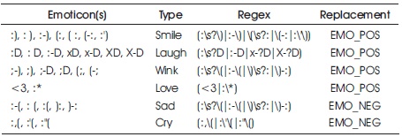
Table 3. List of Emoticons Matched by our Method (Joshi & Deshpande, 2018)
Hashtags are unspaced phrases prefixed by the hash symbol (#) which is frequently used by users to mention a trending topic on Twitter. We replace all the hashtags with the words with the hash symbol. For example, #hello is replaced by hello. The regular expression used to match hashtags is #(\S+).
Retweets are tweets which have already been sent by someone else and are shared by other users. Retweets begin with the letters RT. We remove RT from the tweets as it is not an important feature for text classification. The regular expression used to match retweets is \brt\b.
After applying tweet level pre-processing, we processed individual words of tweets as follows.
Some example tweets from the training dataset and their normalized versions are shown in Table 4 (Joshi, & Deshpande, 2018).
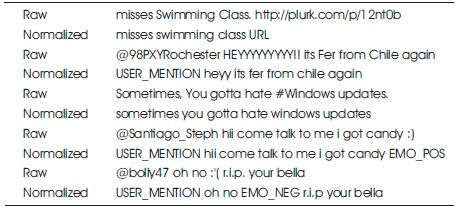
Table 4. Example Tweets from the Dataset and their Normalized Versions (Joshi, & Deshpande, 2018)
We extract two types of features from our dataset, namely unigrams and bigrams. We create a frequency distribution of the unigrams and bigrams present in the dataset and choose top N unigrams and bigrams for our analysis.
Probably the simplest and the most commonly used features for text classification is the presence of single words or tokens in the text. We extract single words from the training dataset and create a frequency distribution of these words. A total of 181232 unique words are extracted from the dataset (Joshi & Deshpande, 2018). Out of these words, most of the words at end of frequency spectrum are noise and occur very few times to influence classification. We, therefore, only use top N words from these to create our vocabulary where N is 15000 for sparse vector classification and 90000 for dense vector classification. The frequency distribution of top 20 words in our vocabulary is shown in Figure 1. We can observe in Figure 2 that the frequency distribution follows Zipf's law which states that in a large sample of words, the frequency of a word is inversely proportional to its rank in the frequency table. This can be seen by the fact that a linear trendline with a negative slope fits the plot of log (Frequency) vs. log (Rank). The equation for the trendline shown in Figure 2 is (Sharma, 2020),
log(Frequency) = −0.78 log(Rank) + 13.31
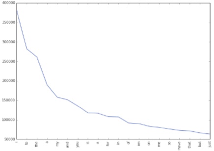
Figure 1. Frequencies of Top 20 Unigrams
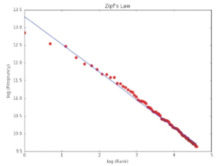
Figure 2. Unigrams Frequencies Follow Zipf's Law
Bigrams are word pairs in the dataset which occur in succession in the corpus. These features are a good way to model negation in natural language like in the phrase – This is not good. A total of 1954953 unique bigrams were extracted from the dataset (Joshi, & Deshpande, 2018). Out of these, most of the bigrams at end of frequency spectrum are noise and occur very few times to influence classification. We therefore use only top 10000 bigrams from these to create our vocabulary. The frequency distribution of top 20 bigrams in our vocabulary is shown in Figure 3.
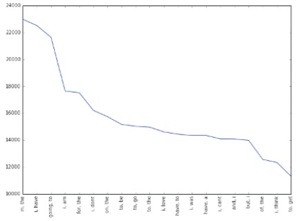
Figure 3. Frequencies of Top 20 Bigrams
After extracting the unigrams and bigrams, we represent each tweet as a feature vector in either sparse vector representation or dense vector representation depending on the classification method.
Depending on whether or not we are using bigram features, the sparse vector representation of each tweet is either of length 15000 (when considering only unigrams) or 25000 (when considering unigrams and bigrams). Each unigram (and bigram) is given a unique index depending on its rank. The feature vector for a tweet has a positive value at the indices of unigrams (and bigrams) which are present in that tweet and zero elsewhere which is why the vector is sparse. The positive value at the indices of unigrams (and bigrams) depends on the feature type we specify which is one of presence and frequency (Sharma, 2020).
Presence: In the case of presence feature type, the feature vector has a 1 at indices of unigrams (and bigrams) present in a tweet and 0 elsewhere.
Frequency: In the case of frequency feature type, the feature vector has a positive integer at indices of unigrams (and bigrams) which is the frequency of that unigram (or bigram) in the tweet and 0 elsewhere. A matrix of such term-frequency vectors is constructed for the entire training dataset and then each term frequency is scaled by the inverse-document-frequency (idf) of the term to assign higher values to important terms. The inverse-documentfrequency of a term t is defined as,
Where, nd is the total number of documents and df (d, t) is the number of documents in which the term t occurs (Raschka & Mirjalili, 2017).
Handling Memory Issues that dealing with sparse vector representations, the feature vector for each tweet is of length 25000 and the total number of tweets in the training set is 800000 which means allocation of memory for a matrix of size 800000 x 25000. Assuming 4 bytes are required to represent each float value in the matrix, this martix needs a memory of 8 x 1010 bytes ≈ (75 GB) which is far greater than the memory available in common notebooks (Ding et al., 2018). To tackle this issue, we used scipy.sparse.lil_matrix data structure provided by Scipy which is a memor y efficient linked list based implementation of sparse matrices. In addition to that, we used Python generators wherever possible instead of keeping the entire dataset in memory.
For dense vector representation, we use a vocabulary of unigrams of size 90000 i.e., the top 90000 words in the dataset. We assign an integer index to each word depending on its rank (starting from 1) which means that the most common word is assigned the number 1, the second most common word is assigned the number 2 and so on. Each tweet is then represented by a vector of these indices which is a dense vector (Sharma, 2020).
Naive Bayes is a simple model which can be used for text classification. In this model, the class cˆ is assigned to a tweet t, where,
In the formula in Equation (1), f represents the i-th feature of i total n features. P(c) and P(f|c) can be obtained through i maximum likelihood estimates (Sharma, 2020).
Maximum Entropy Classifier model is based on the principle of maximum entropy. The main idea behind it is to choose the most uniform probabilistic model that maximizes the entropy, with given constraints. Unlike Naive Bayes, it does not assume that features are conditionally independent of each other. So, we can add features like bigrams without worrying about feature overlap. In a binary classification problem like the one we are addressing, it is the same as using Logistic Regression to find a distribution over the classes. The model is represented by,
Here, c is the class, d is the tweet and λ is the weight vector. The weight vector is found by numerical optimization of the lambdas so as to maximize the conditional probability (Sharma, 2020).
Decision trees are a classifier model in which each node of the tree represents a test on the attribute of the data set, and its children represent the outcomes. The leaf nodes represent the final classes of the data points. It is a supervised classifier model which uses data with known labels to form the decision tree and then the model is applied on the test data. For each node in the tree the best test condition or decision has o be taken. We use the GINI factor to decide the best split. For a given node
where p(j|t) is the relative frequency of class j at node t, and (ni = number of records at child i, n = number of records at node p indicates the quality of the split. We choose a split that minimizes the GINI factor (Sharma, 2020).
Random Forest is an ensemble learning algorithm for classification and regression. Random Forest generates a multitude of decision trees classifies based on the aggregated decision of those trees.
For a set of tweets x1, x2, . . . xn and their respective sentiment labels y1, y2, . . .n bagging repeatedly selects a random sample (Xb , Yb ) with replacement. Each classification tree fb is trained using a different random sample (Xb , Yb ) where b ranges from 1 . . . B. Finally, a majority vote is taken of predictions of these B trees (Sharma, 2020).
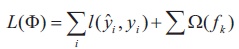
XGBoost is a form of gradient boosting algorithm which produces a prediction model that is an ensemble of weak prediction decision trees. We use the ensemble of K models by adding their outputs in the following manner.
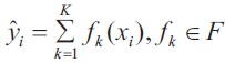
Where, F is the space of trees, xi is the input and yˆi is the final output. We attempt to minimize the following loss function.
where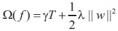
Where, Ω is the regularisation term (Sharma, 2020).
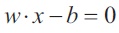
SVM, also known as support vector machines, is a nonprobabilistic binary linear classifier. For a training set of points (xi, yi) where x is the feature vector and y is the class, we want to find the maximum-margin hyperplane that divides the points with yi= 1 and yi= 1.
The equation of the hyperplane is as follow,
We want to maximize the margin, denoted by γ, as follows,
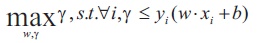
in order to separate the points well (Sharma, 2020).
MLP or Multilayer perceptron is a class of feed-forward neural networks, which has atleast three layers of neurons. Each neuron uses a non-linear activation function, and learns with supervision using backpropagation algorithm. It performs well in complex classification problems such as sentiment analysis by learning non-linear models (Sharma, 2020).
Convolutional Neural Networks or CNNs are a type of neural networks which involve layers called convolution layers which can interpret spacial data. A convolution layers has a number of filters or kernels where it learns to extract specific types of features from the data. The kernel is a 2D window which is slided over the input data performing the convolution operation. We use temporal convolution in our experiments which is suitable for analyzing sequential data like tweets (Sharma, 2020).
Recurrent Neural Networks are a network of neuron-like nodes, each with a directed (one-way) connection to every other node. In RNN, hidden state denoted by h acts t as memory of the network and learns contextual information which is important for classification of natural language. The output at each step is calculated based on the memory ht at time t and current input xt . The main feature of an RNN is its hidden state, which captures sequential dependence in information. We used Long Term Short Memory (LSTM) networks in our experiments which is a special kind of RNN capable of remembering information over a long period of time (Sharma, 2020).
We perform experiments using various different classifiers. Unless otherwise specified, we use 10% of the training dataset for validation of our models to check against overfitting i.e. we use 720000 tweets for training and 80000 tweets for validation. For Naive Bayes, Maximum Entropy, Decision Tree, Random Forest, XGBoost, SVM and Multi- Layer Perceptron we use sparse vector representation of tweets. For Recurrent Neural Networks and Convolutional Neural Networks we use the dense vector representation (Sharma, 2020).
For a baseline, we use a simple positive and negative word counting method to assign sentiment to a given tweet. We use the Opinion Dataset of positive and negative words to classify tweets. In cases when the number of positive and negative words is equal, we assign positive sentiment. Using this baseline model, we achieve a classification accuracy of 63.48% on Kaggle public leaderboard.
We used MultinomialNB from sklearn.naive_bayes package of scikit-learn for Naive Bayes classification. We used Laplace smoothed version of Naive Bayes with the smoothing parameter α set to its default value of 1. We used sparse vector representation for classification and ran experiments using both presence and frequency feature types. We found that presence features outperform frequency features because Naive Bayes is essentially built to work better on integer features rather than floats. We also observed that addition of bigram features improves the accuracy (Sharma, 2020). We obtain a best validation accuracy of 79.68% using Naive Bayes with presence of unigrams and bigrams. A comparison of accuracies obtained on the validation set using different features is shown in Table 5.
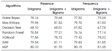
Table 5. Comparison of Various Classifiers which Use Sparse Vector Representation
The nltk library provides several text analysis tools. We use the MaxentClassifier to perform sentiment analysis on the given tweets. Unigrams, bigrams and a combination of both were given as input features to the classifier. The Improved Iterative Scaling algorithm for training provided better results than Generalised Iterative Scaling (Sharma, 2020). Feature combination of unigrams and bigrams, gave better accuracy of 80.98% compared to just unigrams (79.34%) and just bigrams (79.2%).
The nltk library provides several text analysis tools. We use the MaxentClassifier to perform sentiment analysis on the given tweets. Unigrams, bigrams and a combination of both were given as input features to the classifier. The Improved Iterative Scaling algorithm for training provided better results than Generalised Iterative Scaling (Sharma, 2020). Feature combination of unigrams and bigrams, gave better accuracy of 80.98% compared to just unigrams (79.34%) and just bigrams (79.2%).
We use the DecisionTreeClassifier from sklearn.tree package provided by scikit-learn to build our model. GINI is used to evaluate the split at every node and the best split is chosen always. The model performed slightly better using the presence feature compared to frequency (Sharma, 2020). Also using unigrams with or without bigrams did not make any significant improvements. The best accuracy achieved using decision trees have been 68.1%. A comparison of accuracies obtained on the validation set using different features is shown in Table 5.
We implemented random forest algorithm by using RandomForestClassifier from sklearn.ensemble provided by scikit-learn. We experimented using 10 estimators (trees) using both presence and frequency features. presence features performed better than frequency though the improvement has not been substantial. A comparison of accuracies obtained on the validation set using different features is shown in Table 5.
We also attempted tackling the problem with XGBoost classifier. We set max tree depth to 25 where it refers to the maximum depth of a tree and is used to control over-fitting as a high value might result in the model learning relations that are tied to the training data. Since XGBoost is an algorithm that utilises an ensemble of weaker trees, it is important to tune the number of estimators that is used. We realised that setting this value to 400 gave the best result (Sharma, 2020). The best result has been 78.72 which came from the configuration of presence with Unigrams + Bigrams.
We utilise the SVM classifier available in sklearn. We set the C term to be 0.1. C term is the penalty parameter of the error term. In other words, this influences the misclassification on the objective function. We run SVM with both Unigram as well Unigram + Bigram. We also run the configurations with frequency and presence (Sharma, 2020). The best result has been 81.55 which became the configuration of frequency and Unigram + Bigram.
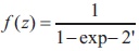
We used Keras with TensorFlow backend to implement the Multi-Layer Perceptron model. We used a 1-hidden layer neural network with 500 hidden units. The output from the neural network is a single value which we pass through the sigmoid non-linearity to squish it in the range [0, 1] (Sharma, 2020). The sigmoid function is defined by
The output from the neural network gives the probability Pr (positive tweet) i.e. the probability of the tweets sentiment being positive. At the prediction step, we round off the probability values to convert them to class labels 0 (negative) and 1 (positive). The architecture of the model is shown in Figure 4. Red hidden layers represent layers with sigmoid non-linearity. We trained our model using binary cross entropy loss with the weight update scheme being the one defined. We also conducted experiments using SGD+ Momentum weight updates and found out that it takes too long to converge. We ran our model up to 20 epochs after which it began to overfit. We used sparse vector representation of tweets for training. We found that the presence of bigrams features significantly improved the accuracy.
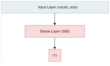
Figure 4. Architecture of the MLP Model
We used Keras with TensorFlow backend to implement the Convolutional Neural Network model. We used the dense vector representation of the tweets to train our CNN models. We used a vocabulary of top 90000 words from the training dataset. We represent each word in our vocabulary with an integer index from 1 . . . 90000 where the integer index represents the rank of the word in the dataset. The integer index 0 is reserved for the special padding word. Further each of these 90000+1 words is represented by a 200 dimensional vector. The first layer of our models is the Embedding layer which is a matrix of shape (v + 1) d where v is vocabulary size (=90000) and d is the dimension of each word vector (=200). We initialize the embedding layer with random weights from (0, 0.01). Each row of this embedding matrix represents the 200 dimensional word vector for a word in the vocabulary. For words in our vocabulary which match GloVe word vectors provided by the StanfordNLP group, we seed the corresponding row of the embedding matrix from GloVe vectors. Each tweet i.e. its dense vector representation is padded with 0s at the end until its length is equal to max_length which is a parameter we tweak in our experiments. We trained our model using binary cross entropy loss with the weight update scheme being the one defined. We also conducted experiments using SGD + Momentum weight updates and found out that it takes longer (100 epochs) to converge compared to validation accuracy equivalent to Adam. We ran our model up to 10 epochs. Using the Adam weight update scheme, the model converges very fast (4 epochs) and begins to overfit badly after that. We, therefore, use models from 3rd or 4th epoch for our results (Sharma, 2020). We tried four different CNN architectures which are which are discussed in subsequent subsections.
1-Conv-NN: As the name suggests, this is an architecture with 1 convolution layer. We perform temporal convolution with a kernel size of 3 and zero padding. After the convolution layer, we apply relu activation function (which is defined as f (x) = max (0, x)) and then perform Global Max Pooling over time to reduce the dimensionality of the data. We pass the output of the Global Max Pool layer to a fullyconnected layer which then outputs a single value which is passed through sigmoid activation function to convert it into a probability value. We also added dropout layers after the embedding layer and the fully- connected layer to regularize our network and prevent it from overfitting. We use a tweet max_length of 20 in this network with a vocabulary of 80000 words.
The complete architecture of the network is embedding_layer (800001×200) → dropout (0.2) → conv_1 (500 filters) → relu→ global_maxpool→ dense (500) → relu → dropout (0.2) → dense(1) → sigmoid as shown in Figure 5. Green layers indicate relu activation while red indicates sigmoid.
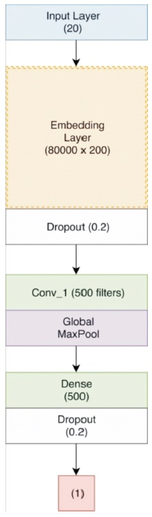
Figure 5. Neural Network Architecture with 1 Conv Layer (Sharma, 2020)
2-Conv-NN: In this architecture we increased the vocabulary from 80000 to 90000. We also increased the dropout after embedding layer to 0.4 and that after the fully connected layer to
0.5 to further regularize the network and thus prevent overfitting. We changed the number of filters in the first convolution layer to 600 and added another convolution layer with 300 filters after the first convolution layer. We also replaced the Global Max Pool layer with a Flatten layer as we believed some features of the input tweets got lost while max pooling. We also increased the number of units in the fully-connected layer to 600. All of these changes allowed the network to learn and regularize better thereby improving the validation accuracy.
The complete architecture of the network is embedding_layer (900001×200) → dropout (0.4) → conv_1 (600 filters) → relu → conv_2 (300 filters) → relu → flatten → dense (600) → relu → dropout (0.5) → dense (1) → sigmoid as shown in Figure 6.
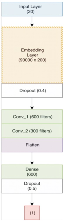
Figure 6. Neural Network Architecture with 2 Conv Layers
3-Conv-NN: In this architecture we added another convolution layer with 150 filters after the second convolution layer.
The complete architecture of the network is embedding_layer (900001×200) → dropout (0.4) → conv_1 (600 filters) → relu → conv_2 (300 filters) → relu → conv_3 (150 filters) → relu → flatten → dense (600) → relu → dropout (0.5) → dense (1) → sigmoid as shown in Figure 7.
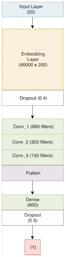
Figure 7. Neural Network Architecture with 3 Conv Layers
4-Conv-NN: In this architecture, we added another convolution layer with 75 filters after the third convolution layer. We also increased max_length of the tweet to 40 going by the fact that the length of largest tweet in our preprocessed dataset is about 40 words.
The complete architecture of the network is embedding_layer (900001×200) → dropout (0.4) → conv_1 (600 filters) → relu → conv_2 (300 filters) → relu → conv_3 (150 filters) → relu → conv_4 (75 filters) → relu → flatten → dense(600) → relu → dropout(0.5) → dense(1) → sigmoid as shown in Figure 8.
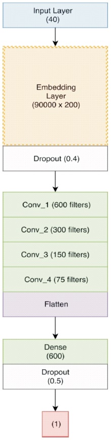
Figure 8. Neural Network Architecture with 4 Conv Layers
We notice that each successive CNN model is better than the previous one with 1-Conv-NN, 2-Conv-NN, 3-Conv-NN and 4-Conv-NN achieving accuracies of 82.40, 82.76, 82.95 and 83.34 respectively on Kaggle public leaderboard.
We used neural networks with LSTM layers in our experiments. We used a vocabulary of top 20000 words from the training dataset. We used the dense vector representation for training our models. We pad or truncate each dense vector representation to make it equal to max_length which is a parameter we tweak in our experiments (Sharma, 2020). The first layer of our network is the Embedding layer which has been described. We test two different types of LSTM models.
In these models, we use a word embedding dimension of 32 and train the embeddings from scratch. The embedding layer is followed by an LSTM layer where we experimented with different number of LSTM units. The LSTM layer is followed by a fully-connected layer with 32 units and relu activation. Finally, the output is a single value with sigmoid activation. We also add dropouts of 0.2 after embedding layer and the penultimate layer to regularize the network.
In these models, we use a word vector dimension of 200 instead and seed it with GloVe word vectors provided by the StanfordNLP group. The word embeddings are fine tuned during the course of training (Pennington, 2014). We follow the embeddings layer with an LSTM layer which is followed by a fully-connected layer with relu activation. Finally, the output is a single value with sigmoid activation. We add dropouts of 0.4 and 0.5 after embeddings layer and the penultimate layer respectively to further regularize the network.
We experimented with different values of LSTM and fullyconnected units and the results are summarized in Table 6. The architecture of our best performing LSTM-NN is shown in Figure 9.
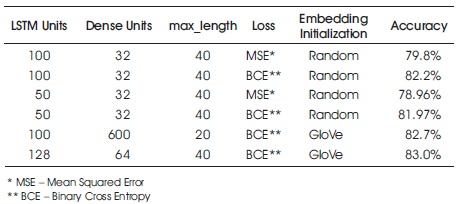
Table 6. Comparison of Different LSTM Models
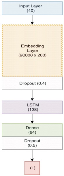
Figure 9. Architecture of Best Performing LSTM-NN
We experimented with both Adam optimizer and SGD with momentum for training our networks and found that Adam worked better and converges faster. We trained our model using mean_squared_error and binary_cross_entropy loss. We found that binary_cross_entropy worked better than mean_squared_error which is expected to give binary classification problem. The results from various different LSTM models are summarized in Table 6. We obtain best accuracy of 83.0% among the different LSTM models.
In a quest to further improve accuracy, we developed a simple ensemble model. We extracted 600 dimensional feature vectors for each tweet from the penultimate layer of our best performing 4-Conv-NN model. Each tweet is now represented by a 600 dimensional feature vector. We use these features to classify the tweets using a linear SVM model with C=1. We classify the tweets using this SVM model. We then take the majority vote of predictions from the following 5 models.
The accuracies from each of these individual models and their majority voting ensemble are shown in Table 7. The flowchart of ensemble is shown in Figure 10.
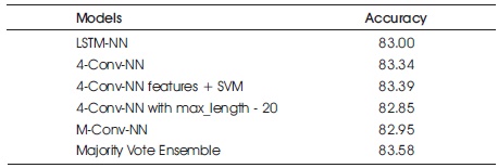
Table 7. Models used for Ensemble and their Accuracies on Kaggle Public Leaderboard
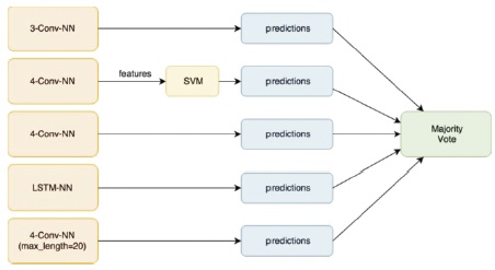
Figure 10. Flowchart of Majority Voting Ensemble
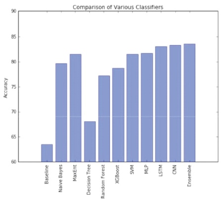
Figure 11. Comparison of Accuracies of Various Models
The provided tweets were a mixture of words, emoticons, URLs, hastags, user mentions, and symbols. Before training, we pre-process the tweets to make it suitable for feeding into models. We implemented several machine learning algorithms like Naive Bayes, Maximum Entropy, Decision Tree, Random Forest, XGBoost, SVM, Multi-Layer Perceptron, Recurrent Neural Networks and Convolutional Neural Networks to classify the polarity of the tweet. We used two types of features namely unigrams and bigrams for classification and observed that augmenting the feature vector with bigrams improved the accuracy. Once the feature has been extracted it is represented as either a sparse vector or a dense vector. It has been observed that presence in the sparse vector representation recorded a better performance than frequency.
Neural methods performed better than other classifiers in general. Our best LSTM model achieved an accuracy of 83.0% on Kaggle while the best CNN model achieved 83.34%. The model which used features from our best CNN model and classified using SVM performed slightly better than only CNN. We finally used an ensemble method taking a majority vote over the predictions of 5 of our best models achieving an accuracy of 83.58% (Krishna et al., 2020).
Handling Emotion Ranges: We can refine and train our models to deal with a variety of emotions. Tweets do not always have a positive or negative tone; they may have no emotion at times, i.e., they are neutral.
Grading the Text: Sentiment can also be graded, such as “this sentence is nice”, “is positive”, “but this sentence is exceptional”, “is a little more upbeat than the first”. As a result, we may categorise the sentiment into ranges, such as -2 to +2.
Using Symbols: As part of pre-processing, we removed most symbols like commas, full stops, and exclamation points during pre-processing. In sentimental analysis, these symbols could be useful in determining the sentiment of a text.
On Twitter, we obtained results for sentiment analysis. We reported an overall increase for two rating tasks: binary, positive versus negative, and triple positive against negative versus neutral, using the created unigram model as our baseline. Based on the review conducted in this paper, we conclude that 4-Conv-NN features + SVM produced maximum accuracy based on majority vote ensemble on the Kaggle dataset. We immediately come to the conclusion that sentiment analysis of Twitter data is not dissimilar to sentiment analysis of other forms of data. In future, more advanced linguistic analyses, such as parsing, semantic analysis, and subject modelling will be studied.