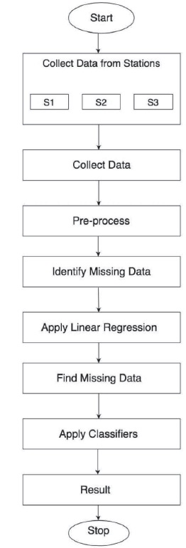
Figure 1. Flow of Control
Though Machine Learning is a discipline in software engineering, it contradicts from the usual computing styles. In usual computing style, algorithms are sets of expressly programmed instructions utilized by computers to compute or solve the problem. Machine learning algorithms rather take into consideration for computers to prepare on information sources and utilize measurable examination keeping in mind the end goal to yield esteems that fall inside a particular range. This paper addresses five most commonly used classification algorithms, such as Logistic Regression, Naïve Bayes, K-Nearest Neighbors, Decision Tree, and Support Vector Machine. It aims to recover the incomplete sensed data of an IoT environment and proves that Linear Regression is the best suited for data recovery.
With access to immense volumes of information, chiefs oftentimes make determinations from information archives that may contain information quality issues, for different type of reasons. Missing information, that is, fields for which information is inaccessible or fragmented is an essential issue since it can lead the investigators to make off-base inferences. At the point when information is extricated from an information distribution center or database (a typical event while accumulating information from various sources), it commonly goes through a purifying procedure to decrease the occurrence of absent or uproarious qualities quite far.
Some missing information traits cannot be settled in light of the fact that the database administrator might not have any method for knowing the esteem that is absent or fragmented, as would happen (Quang & Miyoshi, 2008). Now, the database chief may evacuate the records with missing information, at the loss of the intensity of the other information qualities that are contained in these records, or to furnish the dataset with missing information records. Information approvals might miss for a different types of reasons, falling into two general classifications: Missing At Random (MAR) and Missing Not At Random (MNAR). In the MAR case, the frequency of missing data cannot be anticipated in view of other information, while in the MNAR case, there is an example among the missing information records. For MAR situations, there exist techniques for assessing, or ascribing the missing qualities. The rate of missing information, anyway regularly falls into the missing not at random classification; that is there is an inclination in the event of invalid or missing qualities (Mnih & Salakhutdinov, 2008).
Machine Learning is a part of Artificial Intelligence (AI), where the structure of information is understood by the machine which comprehends the information into models that can be easily understood by humans. Machine learning makes personal computers to prepare information inputs, use true examination, and outputs information that falls inside a particular category. Along these lines, Machine Learning facilitates of personal computers in building models from test data in order to robotize fundamental frames in perspective of data inputs. The reason for this exploration is to assemble the five most generally utilized classification algorithms (Kumar & Pranaw, 2017) along with the python code: Logistic Regression, Naïve Bayes, K-Nearest Neighbours, Decision Tree, and Support Vector Machine.
Definition: Logistic regression is a machine learning algorithm for classification. In this algorithm, the probabilities portraying the conceivable results of a solitary preliminary are demonstrated utilizing a logistic function.
Advantages: Logistic regression is intended for this reason (classification), and is most helpful for understanding the impact of a few autonomous factors on a solitary result variable.
Disadvantages: Works just when the anticipated variable is binary, accept all indicators are autonomous of each other and expect information is free of missing values.
Definition: Naive Bayes algorithm based on Bayes' theorem with the suspicion of autonomy between each combination of highlights. Naive Bayes classifiers function admirably in some true circumstances for example document classification and spam filtering.
Advantages: This algorithm requires a little measure of training data to evaluate the fundamental parameters. Naive Bayes classifiers are greatly quick contrasted with more modern strategies.
Disadvantages: Naive Bayes is known to be a terrible estimator.
Definition: Neighbours based classification is a kind of sluggish learning as it doesn't endeavor to build a general inside model, yet just stores examples of the training data. Classification is processed from a basic share vote of the k nearest neighbors of each point.
Advantages: This algorithm is easy to execute, powerful too noisy training data, and successful if training data is large.
Disadvantages: Need to decide the estimation of K and the calculation cost is high as it needs to compute the separation of each case to all the preparation tests.
Definition: Given an information of characteristics with its classes, a decision tree creates an arrangement of principles that can be utilized to classify the data.
Advantages: Decision Tree is easy to comprehend and envision, requires little information readiness, and can deal with both numerical and clear-cut information.
Disadvantages: Decision tree can make complex trees that do not sum up well, and decision trees can be temperamental in light of the fact that little varieties in the information may result in a totally unique tree being produced.
Definition: Support Vector Machine is a portrayal of the training data as focuses on space separated into categories by a clear gap that is could be expected under the circumstances. Same space is used to map the new examples.
Advantages: Effective in high dimensional spaces and uses a subset of preparing focuses in the decision function so it is additional memory proficient.
Disadvantages: The algorithm does not specifically give likelihood evaluates. These are ascertained utilizing a costly five-fold cross-validation.
An approach for recovering missing data in IoT (Internet of Things) implements a K-means clustering algorithm to isolate sensors into various gatherings. The principal objective of clustering is to guarantee that sensors inside one gathering will have similar patterns of measurement. After clustering, a Probabilistic Matrix Factorization (PMF) algorithm is applied within each cluster (Srivastava et al., 2016). Since the sensors are assembled by likeness in their estimations, it is conceivable to recuperate missing sensor information by investigating examples of neighboring sensors. To enhance the execution of information recuperation, the PMF algorithm is upgraded by normalizing the information and restricting the probabilistic distribution of random feature matrices.
Drawbacks in K-means:
If anyone of these four assumptions is violated, then kmeans will fail.
Numerous articles have been studied to manage the missing data problem (Jiang & Gruenwald, 2007), and a ton of programming have been produced in view of these techniques. A portion of the techniques thoroughly erase the missing data before dissecting them, similar to list insightful and match savvy erasure, while some different strategies center around evaluating the missing data in light of the accessible data. The most prevalent factual estimation strategies incorporate mean substitution, imputation by regression, hot-deck imputation, cold deck imputation, Expectation Maximization (EM), maximum likelihood, multiple imputations, and Bayesian analysis.
Multiple Imputation using Gray-system-theory and Entropy-based on Clustering (MIGEC) is a new hybrid data completing method. Its strategy includes two steps. Firstly, it forms clusters of information with the non-missing data. Secondly, computation over imputed values is done using data entropy of proximal loss for each cluster formed in the first step.
Various complexities can be measured by developing techniques that involve feature selection and classification. The main intention of developing these techniques is to emphasize on methodologies that highly affect transience timeframe and develop paradigms that adapt to missing values. To deal with the missing value imputation algorithms such as K-means clustering and Hierarchical Clustering were already in existence. These approaches deal with similarities that are uncovered. They had connected the programming techniques to advance and process the matrices of the clinical data set which are having missing information. Three feature selection techniques; t-Test, entropy Ranking, and Nonlinear Gain Analysis (NLGA) are utilized to distinguish the most widely recognized highlights inside the data set.
Under this method, the data set segments are skewed and the imputed values have the same distributional shape as the observed data. The hot deck includes two phases. In the first phase, the data set is divided into clusters (Li & Parker, 2008). In the second phase, the missing data in the data send are linked to one cluster. Then mean or mode of the attributes within the cluster are calculated. Here, the donor is chosen from the same data source which contradicts with Cold Deck Imputation where the donor is chosen from other data source.
Characterizing an arrangement of values that are nearest to the predicted values and picking one value out of that set at random for imputation can represent randomization. This Imputation strategy joins the parametric and non-parametric techniques which attribute the missing values by its nearest-neighbor donor in which the distance for the missing values are figured from the normal estimations of the missing data.
Linear regression is the method used for numeric variables and works with linear functions based on probability whereas Logistic Regression is used for unqualified (Uncategorized) data and uses logistic functions (Williams et al., 2005) based on probability. The predictive regression imputation utilizes auxiliary variables (Xi) to trace the missing values (Yi). The issue of missing data from sensors has been generally known in Wireless Sensor Networks (WSNs) for quite a while (Kulakov & Davcev, 2005). There are numerous answers to recuperating missing data in WSNs, however, every one of them requires an immediate connection between sensor nodes. A spatial-temporal replacement scheme to recover missing data by considering the nature of a WSN (Quang & Miyoshi, 2008). This approach utilizes neighboring sensor readings if an objective hub has no readings. In this way, if the neighboring hub identifies a change, it is likely that there are a few changes in nature.
Another comparable approach is the recovery of missing values by using data from neighboring nodes. However, this approach is more advanced because they introduced a window-association rule-mining algorithm to determine the sensor node that is related to the sensor node with the missing value. In any case, this approach decides the connection between just two sensor nodes. Keeping in mind the end goal to overcome this limitation, a data estimation technique (Fekade et al., 2018) by utilizing closed item set-based association rule mining that determines relations between two or more sensors to recover missing values was introduced. The most straightforward technique is mean substitution, which imputes the average value of all non-missing values to replace the missing values.
Filling in or “Impute” missing values is a new approach that is implemented in this paper rather than force out factors or perceptions with missing data. A wide variety of imputation methodologies can be used that range from easy level to arbitrary level. These methods keep the full sample size with favors for accuracy and foregone conclusion. However, they can result in different kinds of bias (Le, 2005). Use of single imputation strategy results in few numbers of standard errors of estimates.
The insight here is to identify significant ambiguity about the missing values. But the choice of single imputations was a substance puts on a show to think about the bonafide motivation with convictions. The most effortless approach to substitute each missing value with the mean of the observed values of that variable. This approach is implemented in mean imputation. But this method has its own disadvantages such as distortion in distribution for the variable, prompting difficulties with rundown measures including underestimates of the standard deviation. It also alters the relationship between variables by making estimates of the correlation towards zero.
Least demanding approach to attribute is to supplant each missing value with the mean of the watched values for that variable. Shockingly, this system can extremely mutilate the distribution for this variable, leading to complications with rundown measures including, notably, thinks little of the standard deviation. Additionally, mean imputation mutilates relationships between variables by “pulling” evaluations of the correlation toward zero. The flow of control can be observed in Figure 1.
Figure 1. Flow of Control
Linear regression is a typical Statistical Data Analysis technique (Pigott, 2001). It is utilized to decide the degree to which there is a direct connection between a dependent variable and at least one autonomous variables. There are two sorts of linear regression, simple linear regression, and multiple linear regression.
In basic linear regression, a solitary independent variable is utilized to anticipate the estimation of a dependent variable. In various linear regressions, at least two autonomous variables are utilized to foresee the estimation of a dependent variable. The distinction between the two is the number of free variables. In two cases, there is just a solitary ward variable.
Linear regression has numerous practical uses. Most applications can be categorized as one of the two general classifications:
Missing data can happen on account of no data is accommodated at least one things or for an entire unit ("subject"). A few things will probably create a nonresponse than others.
There are distinctive assumptions about missing data mechanisms:
Suppose variable Y has some missing values, we will state that these values are MCAR if the likelihood of missing data on Y is irrelevant to the estimation of Y itself or to the estimations of some other variable in the data set. However, it does allow for the likelihood that “missingness” on Y is neither relies neither upon Y nor on some other variable X.
It means that there is no connection between the missingness of the data and any values, watched or missing. Those missing data points are an arbitrary subset of the data. There is nothing deliberate going on that makes some data more prone to be missing than others.
The likelihood of missing data on Y is disconnected to the value of Y in the wake of controlling for other variables in the analysis (say X). On another hand, Missing value (Y) relies upon X, yet not Y.
Means there is an efficient relationship between the inclination of missing values and the observed data, however not the missing data. Regardless of perception is missing has nothing to do with the missing values, yet it has to do with the values of an individual's watched variables.
Missing values rely upon in unobserved values. On another hand, the likelihood of a missing value relies upon the variable that is missing.
MNAR is called “non-ignorable” in light of the fact that the missing data mechanism itself must be demonstrated as you manage the missing data. You have to incorporate some model for why the data are missing and what the feasible qualities are “Missing completely at Random” and “Missing at Random” are both viewed 'ignorable' in light of the fact that we don't have to incorporate any information about the missing data itself when we manage with the missing data.
Initially, an arbitrary dataset was taken as input, which comprises some missing or null values. Here the principle point is to locate the missing values in that dataset utilizing linear regression. By applying linear regression to the dataset it replaces the null values. By figuring mean to each column in a dataset the null value should be supplanted by that mean value in the dataset, in the wake of recuperating the null values now supply that new dataset to different classifiers like logistic regression, decision tree classifier, SVM, linear discrimination analysis, K-neighbour classifier to calculate the accuracy.
Every classifier partitions the data set into two sets i.e., a training set and a test set. We take test set data of each classifier and ascertain mean and variance. In the wake of figuring the mean and variance which classifier gets the most elevated mean value will have good accuracy among other classifiers.
Guido van Rossum was instrumental in developing Python programming language was developed in the late eighties and early Nineties at National Research Institute of Mathematics and Computer Science, Netherlands (Downey, 2015). It can be treated as a mix of best features of various programming languages, such as ABC, Algol – 68, C, C++, Modula – 3, Smalltalk, and other shell and scripting languages. Python is made available to the general public under the General Public License (GPL).
Besides the above-said features python also has its advantages which were mentioned below.
Figure 2 illustrates the primary dataset that is taken as input to the implemented system. The dataset contains information on air pollution with null values. The parameters of the air pollution data are location id, temperature, humidity, wind, wind direction, gas, pressure, air quality. From Figure 3, null values are replaced with NAN to trace them easily in the input primary dataset.
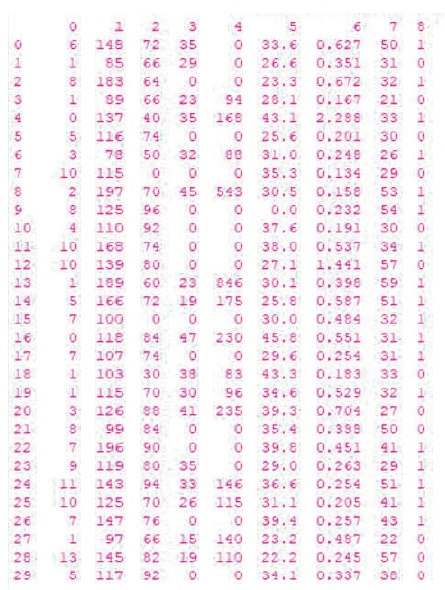
Figure 2. Primary Data Set with Null Values

Figure 3. Null Values placed with “NAN”
From Figure 4, the final dataset is calculated values by applying linear regression. Here the authors have used Python simulation tool to calculate the missing data. First, we have to install the NumPy and Pandas packages in Python. These packages are used to import the dataset in the program. After that, linear regression is applied to the dataset. In Python, linear regression is an inbuilt feature it will generate the nearby values of the original dataset by using a dependent variable.
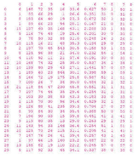
Figure 4. Final Data Set with Calculated Values
From Figure 5, the calculated mean values for different classifiers are logistic regression, linear discrimination analysis, classification, and regression tree, k nearest neighbor, Naïve Bayes, and support vector machine.
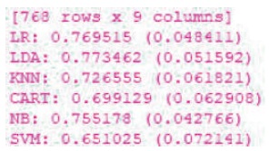
Figure 5. Different Classifiers Mean Values
From Figure 6, the comparison graph among the different classifiers are available by calculating their respective means. The logistic regression classifier has the highest mean value among the other classifier. Logistic regression classifier shows the better result for this dataset.
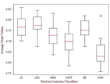
Figure 6. Different Classifiers Mean Graph
This paper presents a technique for predicting missing values of sensor node as well as to maintain and improve the efficiency. Data loss is unavoidable in a wireless network, and it causes many complications in its various applications. To comprehend and locate the appropriate procedures for building up the model for examining the impact of missing instances in a dataset are carried out. Besides this, the key factor is to comprehend the idea of the dataset with a specific end goal to pick the reasonable procedure. The implemented Linear Regression aims to predict the missing data with less error and it has also been effective even when a high volume of data is missing.
Future work incorporates execution of Random forests or random decision forests are a troupe learning method for classification, regression, and different undertakings, that work by building a large number of decision trees at training time and yielding the class that is the mode of the classes (classification) or mean prediction (regression) of the individual trees. Random decision forests adjust for decision trees' habit of overfitting into their training set.