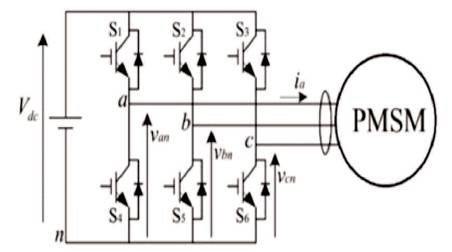
Figure 1. Block diagram of VSI fed PMSM
This paper contains the modelling and simulation result of classical (vector control) field oriented control and Space Vector Pulse Width Modulation (SVPWM) voltage source inverter fed Permanent Magnet Synchronous Motor (PMSM). Permanent magnet motor drives are used in many industrial applications such as driving the robot and CNC machine tool. The precise control of a permanent magnet motor drive is not easy due to the presence of nonlinearities in Permanent magnet motor servo systems, parameter and load torque variations. Advanced pulse width modulation and control techniques, such as Space Vector Pulse Width Modulation and Field Oriented Control, have been used for the closed-loop control of the system. Next, a model of diode-rectified two-level voltage source inverter is developed for simulations. A comparative study of indirect space vector modulated direct two-level voltage source inverter converter and space vector modulated diode-rectified two-level voltage source inverter is given in terms of input/output waveforms to verify that the converter fulfills the two-level voltage source inverter operation.
Recently, the Permanent Magnet Synchronous Motor (PMSM) has been widely employed in our life and industrial control because of its several inherent advantages. Generally speaking, high-precision and high-resolution sensors are necessary to obtain accurate position and speed information to control PMSM precisely. While, speed or position sensors require the additional mounting space, increase the cost and the complexity of the system as well as reduce the reliability of the system.
A Permanent Magnet Synchronous Motor (PMSM) becomes increasingly popular for high resolution servo motor drives such as CNC machine tools and industrial robots. A Permanent magnet synchronous motor features low noise, low inertia, high efficiency, robustness and low maintenance cost. To achieve high dynamic performance and high precision, many researchers have presented various control methods, e.g. neural network control [2-4], robust control [6], sliding mode control [3], adaptive control [5,7,8,9,10] and sensor less control [17].
Most of the previous control methods have been developed under the assumption of availability of knowledge on the PMSM parameters. However, the PM synchronous motor is subject to system parameter variations and external disturbances, and thus most of the previous control methods cannot assure the closed-loop system stability under uncertainties such as motor parameter and load torque variations.
Vector control offers superior performance when compared to scalar control. Vector control eliminates almost all the disadvantages of scalar control. The main idea of vector control is to control not only the magnitude and frequency of the supply voltages, but also the angle. With other words said the magnitude and angles of the space vectors are controlled. There are different kinds of vector controls, the two most commonly used being DTC (Direct Torque Control) and FOC (Field-Oriented Control) [12].
The space vector modulation technique is somewhat similar to the sine+3rd harmonic PWM technique, but the method of implementation is different. The concept of voltage space-vector, in analogy with the concept of flux space-vector as used in three-phase AC machine. The stator windings of a 3-phase AC machine (cylindrical rotor), when fed with a three-phase balanced current produce a resultant flux space-vector that rotates at synchronous speed in the space. The flux vector due to an individual phase winding is oriented along the axis of that particular winding and its magnitude alternates as the current through it is alternating. The magnitude of the resultant flux due to all three windings is, however, fixed at 1.5 times the peak magnitude due to individual phase windings. The resultant flux is commonly known as the synchronously rotating flux vector [11], [13] .
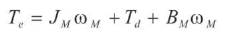
Figure 1 shows the basic block diagram of open loop controlled inverter fed PMSM drive. If DC supply is available for drive, an AC machine inverter fed system is used to drive the motor.
Figure 1. Block diagram of VSI fed PMSM
The main objective of this research is to improve the performance of a PMSM drive system by achieving more precise speed tracking and smooth torque response by implementing a Space Vector Pulse Width Modulation algorithm for employing their superior performance.
The overall objectives to be achieved in this study are:
The following assumptions are considered before establishing the mathematical modeling of permanent magnet synchronous motor:
The mathematical model is similar to that of the wound rotor synchronous motor. Since there is no external source connected to the rotor side and variation in the rotor flux with respect to time is negligible, there is no need to include the rotor voltage equation. Rotor reference frame is used to derive the model of the PMSM [15,19].
The electrical dynamic equation in terms of phase variable can be written as:
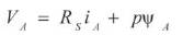
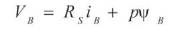
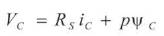
Where VA , VB and VC are instantaneous phase voltage, iA , iB and iC are instantaneous phase current, RS is phase resistant, p is derivative operator, ΨA, ΨB and ΨC are rotor coupling flux linkage.
While the flux linkage equations are:
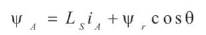
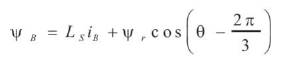
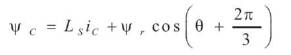
Where, Ls is Phase Inductance.
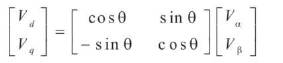
The transformation from 3-phase to 2-phase quantities can be written in matrix form as:
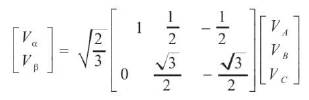
where Vα and Vβ are orthogonal space phasors.
For motor control applications, use the rotating-reference frame to control currents in the so-called d–q system of reference. Figure 2 shows the space vector of d-q coordinates.
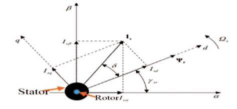
Figure 2. Space Vector Diagram of PMSM Motor in Stationary α-β and Rotating d−q Coordinates
Co-ordinate transformation helps to solve 3 phase system. The a-b-c currents onto a pair of axes which is called as the d and q axes or d-q axes. In making these projections, we want to obtain expressions for the components of the stator currents in phase with the d and q axes, respectively. Although we may specify the speed of these axes to be any speed that is convenient for us, we will generally specify it to be synchronous speed, ωs . Figure 3 shows the generalized 3 phase to two phase rotating reference frames.
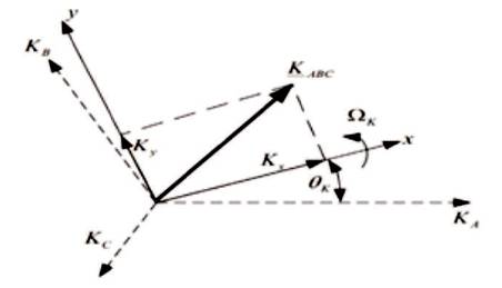
Figure 3. Stator Fixed Three Phase Axes (A, B, C) and General Rotating Reference Frame
According to above transformation, d-q/abc transformation may be written as:
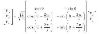
Simple transformed equations are:
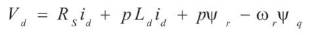
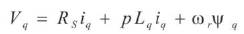
Where Ld and Lq are called d-and q-axis synchronous inductances respectively, ωr is motor electrical speed.
The produced torque Te which is power divided by mechanical speed can be represented as:
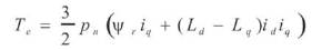
Where, Pn is pole Logarithm.
It is apparent from the above equation that the produced torque is composed of two distinct mechanisms. The first term corresponds to “the mutual reaction torque” occurring between iq and the permanent magnet, while the second term corresponds to “the reluctance torque” due to the difference in d- and q-axis reluctance [15] . Note that Ld =Lq =Ls for the motor, so an expression for the torque generated by a PMSM is:
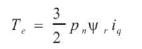
In the presence of a d-axis stator current, the d-axis and qaxis currents are not decoupled, and the model is nonlinear, which is shown in the torque equation (12). Under the assumption that id= 0, the system becomes linear and thus vector control of PMSM provides approximate desired dynamic characteristics.
In general, the mechanical equation of the PMSM can be represented as
where,
ωm =rotor angular speed,
JM =motor moment inertia constant,
BM =damping coefficient,
Td =torque of the motor external load disturbance,
Te =electromagnetic torque.
The electromagnetic torque of the PMSM is not only produced by the permanent magnet flux, but also by the reluctance difference in rotor d- and q-axes. Figure 4 shows mathematical block diagram of permanent magnet synchronous motor.
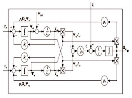
Figure 4. PM Synchronous Machine in Rotating
Electromagnetic torque as cross vector product of the stator flux linkage and current space vectors or rotor and stator flux linkages is independent of coordinate system selected. Therefore, it can be expressed in stationary (α-β) or rotated (d-q) coordinates.
The SVPWM consists of four major processes [1,14,16]:
Figure 5 shows the process of generation of SVPWM. Figure 5 shows the space vector of three-phase Voltage Source Inverter (VSI) divided into six sectors based on the six fundamental vectors VX (x=1, 2, 3…, 6). Any voltage vectors in this vector space can be synthesized by two fundamental vectors VX and VX+1 . For example, the voltage vector in sector I can be represented as a combination of active vectors V1 and V2 . Within a switching cycle Ts, the components for each fundamental vector Vs is related to the occupied time Tn and unoccupied time of the null vectors. The locus of the maximum Vs is represented by the envelope of the hexagon formed by the basic space vectors in Figure 6. Thus, the magnitude of Vs must be limited to the shortest radius of this envelope when Vs is revolving, which gives a maximum magnitude of  for Vs .
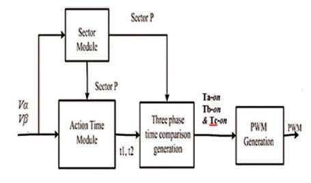
Figure 5. Block Diagram of SVPWM
Figure 6. Sectors of SVPWM
For the computation of sector and vectors, the three phase a-b-c voltage is transformed to α-β reference frame using the Clarke transformations. In Field Oriented Control of PMSM, the α-β voltages are obtained from the d-q voltages [18, 19].
To determine the switching time instants and switching sequence, it is important to know the sector in which the reference vector lies. Following algorithm can be used to determine the sector of the reference output voltage vector. Three intermediate variables are considered as Vref1 , Vref2 and Vref3 [10].
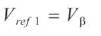
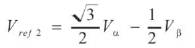
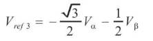
A, B and C are considered as logical variables which takes the values 0 or 1 depending on the conditions:
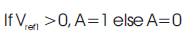
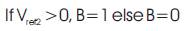

Using the logical variables A, B and C, the variable N is identified as:
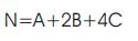
Values of N are used to map the sector (P) where the vector lies, as per Table 1.
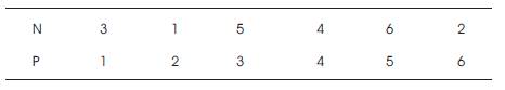
Table 1. Mapping of N to P
The action time of two adjacent basic vectors in a certain sector is defined as t1 and t2 . In traditional SVPWM algorithm, space angles and trigonometric functions are used to calculate the values of t1 and t2 , which makes the process complex. In this method, these values are calculated using Vα and Vβ [1]. Applying the volt-second balance principle to the orthogonal decomposition rates of the basic vectors, t1 and t2 can be mapped from Table 2.
Table 2. Mapping X, Y, Z to T1 and T2
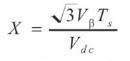
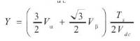
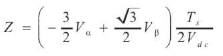
Where X, Y and Z are given by:
Ta, Tb and Tc correspond to the time comparison values of each phase. Intermediate variables Ta-on, Tb-on and Tcon are used to map the comparison values from Table 3.
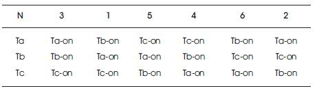
Table 3. Generation of TA , TB and TC
The overall block schematic of FOC of PMSM is shown in Figure 7. In this control system, stator currents ia and ib are measured using electric current sensors, and ic is calculated with the formula ic =–(ia +ib ). The electric currents ia , ib and ic are transformed into the direct component iq , id in the revolving coordinate system through the Clarke and the Park transformations. Then iq , id can be used as the negative feedback quantity of the electric current loop. The deviation between the given speed and the feedback speed ω* is regulated through the speed PI regulator. The output is q axis reference component iq* - torque component, which is used to control the torque. The deviations between iq* , id* and current feedback quantity iq , id is fed to the current PI regulators, and the respective output phase voltage Vq* and Vd* on the d-q revolving coordinate system. Vq* and Vd* are transformed into the stator phase voltage vector component Vα and Vβ , respectively under α-β coordinate system through inverse Park transformation. If the stator phase voltage vector Vα , Vβ and its sector number is known, the voltage Space Vector PWM technique can be used to produce PWM signal to control the inverter, so as to achieve closed-loop control of the PMSM. In the algorithm, id*=0 as there is no excitation in the rotor part for a PMSM. This paper presents the simulation of Field Oriented Control of a surface mounted PMSM using the novel SVPWM. Block Diagram of SVPWM FOC of PMSM Drive is shown in Figure 8.
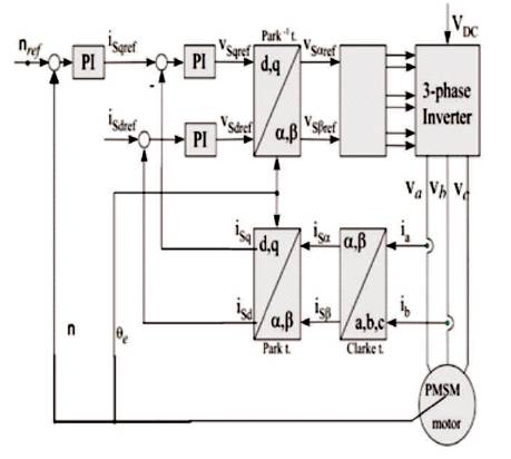
Figure 7. Block Diagram of Classical FOC Controlled PMSM
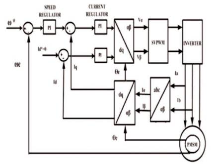
Figure 8. Block Diagram of SVPWM FOC of PMSM Drive
In sector V0 {000} and V7 {111} state, no voltage is generated because of a short circuit situation created. Table 4 shows the different switching vector state and line voltages generated between different phases.
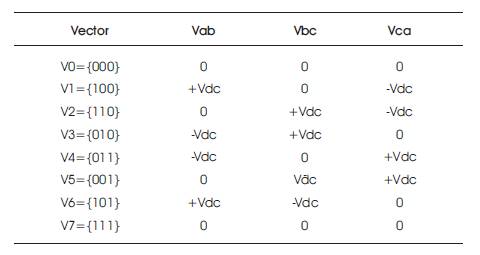
Table 4. SVPWM Switching Technique
Permanent magnet synchronous motor parameters are given in Table 5.
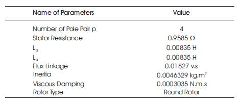
Table 5. Parameters of PMSM
Figures 9 to 11 show the stator current, speed response and electromagnetic torque of classical field oriented control of Permanent Magnet Synchronous Drive (PMSM), respectively.
Figure 9 shows the stator current of classical FOC of PMSM drive. The waveform shows more fluctuation at initial stage.
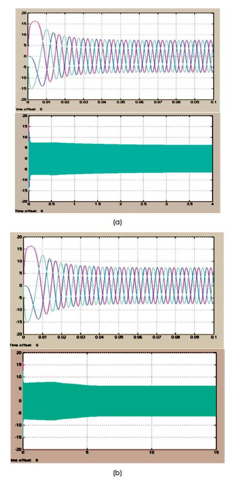
Figure 9. Stator Current of FOC of PMSM for, (a) 300 rpm (b) 500 rpm
Figure 10 shows the speed response of PMSM drive. It shows the speed transient from 0 sec–0.6 sec. At 0.6 sec, the speed reaches at steady state level.
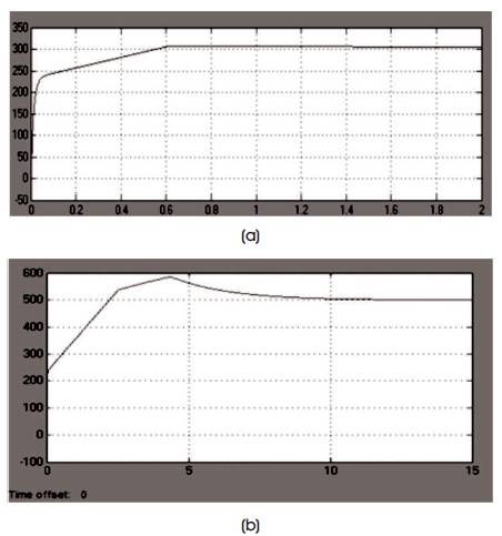
Figure 10. Speed Response of PMSM for, (a) 300 rpm, (b) 500 rpm
Figure 11 shows the electromagnetic torque of PMSM drive. It shows the speed transient from 0 sec–0.6 sec. At 0.6 sec, the electromagnetic torque reaches steady state level.
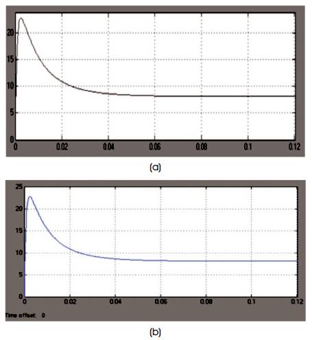
Figure 11. Electromagnetic Torque of PMSM for, (a) 300 rpm, (b) 500 rpm
Figures 12 to 14 show the stator current, speed response, electromagnetic torque of Space Vector Pulse Width Modulated Field Oriented Control of permanent magnet synchronous drive (PMSM).
Figure 12 shows the stator current of Space Vector Pulse Width Modulation FOC of PMSM drive. The waveform shows no fluctuation at initial stage as compared to classical FOC.
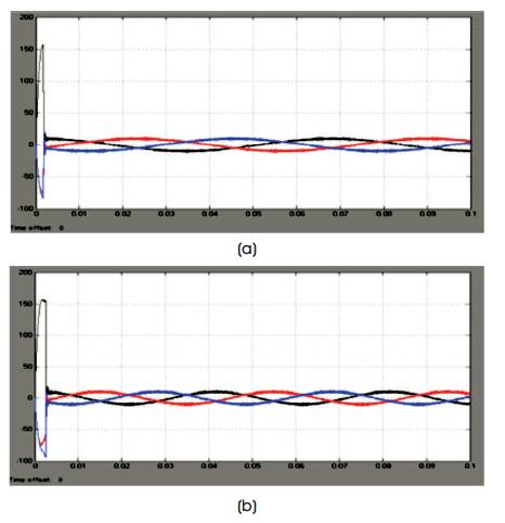
Figure 12. Stator Current of PMSM using SVPWM for, (a) 300 rpm (b) 500 rpm
Figure 13 shows the speed response of PMSM drive. It shows the speed transient from 0 sec–0.011 sec. At 0.011 sec, the speed reaches at steady state level.
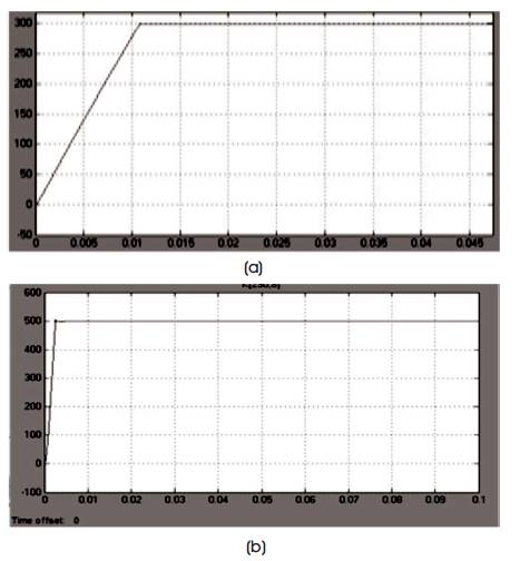
Figure 13. Speed Response of PMSM using SVPWM for, (a) 300 rpm (b) 500 rpm
Figure 14 shows the electromagnetic torque of PMSM drive. It shows the torque transient from 0 sec–0.011 sec. At 0.011 sec, the speed reaches steady state level.
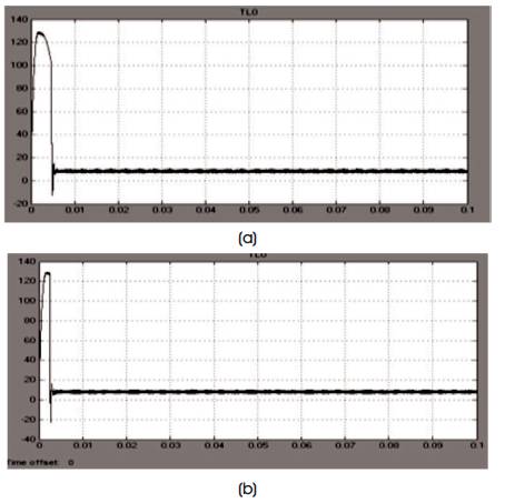
Figure 14. Electromagnetic Torque of PMSM using SVPWM for, (a) 300 rpm (b) 500 rpm
The simulation result of classical controlled PMSM drive and SVPWM controlled PMSM drive shows that for SVPWM controlled drive speed response, electromagnetic torque is better than vector controlled drive. The stator current of SVPWM are not as good as vector controlled PMSM drive. In space vector control, there is less overshoot, low time response and the ripples present in torque is also less. On overall conclusion of PMSM drive, the Space Vector Pulse Width Modulation are better than vector controlled method.
The main advantages of Permanent Magnet (PM) machines are:
Compared with the above mentioned many special features and characteristics of PMSM, it has been found a very interesting subject matter for the present researchers. PMSM drive is maintenance free, which ensures the most efficient operation and it may be operated at improved power factor which may help in improving the overall system power factor and eliminating or reducing utility power factor penalties. From the research over PMSM until now it shows that, in future market PMSM drive could become an emerging competitor for the Induction motor drive in servo application and many industrial applications. So, now there is a great challenge to improve the performance with accurate speed tracking and smooth torque output minimizing its ripple during transient as well as steady state condition such that it may meet the expectation of future market demand.
So, looking out with such a motive, in present work a speed controller having superior performance for speed tracking has been designed as outer loop and a current controller which may provide smooth ripple and less torque response has also been designed as inner loop for closed loop operation of the drive. Modelling and simulation is usually used in designing PM drives compared to building system prototypes because of the cost. Consider having selected all components, the simulation process may start to calculate steady state and dynamic performance and losses would have been obtained if the drive were actually constructed. This practice reduces time, cost of building prototypes and ensures that requirements are achieved. Hence, simulations have helped the process of developing new systems including motor drives, by reducing cost, which is done here in MATLAB/Simulink platform.