[1]

In this paper, a simultaneous approach to choose optimal number of wind based Distributed Generation (DG) units and their locations is proposed with an objective of minimizing annual energy loss in a distribution network. Most of the methods developed so far for optimal allocation of DG units assumed constant DG output and network load profile which is unreal. Optimal DG sizes and locations found with above assumptions would not lead to minimum annual energy loss when employed in realistic scenario where there is uncertainty in the DG output power generation and network loads have a time-varying load profile. In this work, wind based generation units are considered as the DG sources for allocation. In order to gauge the effect of uncertainty in wind power generation and time-varying load profile on optimal DG allocation problem, a meta-heuristic method which employs Harmony Search algorithm is used to solve multiple wind based DG units. Performance and effectiveness of the proposed method is demonstrated by carrying out simulations on 33-bus and 69-bus radial distribution systems. Simulation results indicate that consideration of uncertainty in wind power generation and time varying load profile significantly affects location and size of DG resources in distribution systems.
Distributed Generation (DG) units are small-scale power generation technologies (normally in the range of 3 kW to 10,000 kW) located on-site which provide an alternative to or enhance traditional power system (Ackermann et al., 2001). Liberalization of electricity markets, reduced T&D costs and losses, efficient DG technologies and increased reliability are some of the reasons for increased proliferation of DGs. Major technical benefits of DG are reduced line power losses, voltage profile betterment, enhanced overall energy efficiency and relieved T&D congestion (Rajkumar et al., 2012). However, choosing proper location and size are two important factors to maximize the benefits. To solve optimal location and sizing problem of DG many methods were proposed in recent past.
Acharya et al. (2006) proposed an analytical approach to obtain optimal location and their corresponding optimal DG size to minimize power loss which is based on exact loss formula. This method is applicable for single DG unit allocation only. Results obtained were compared with loss sensitivity method and exhaustive load flow method. Gozel and Hocaoglu (2009) employed loss sensitivity factor based on equivalent current injection method to determine optimum location and size of DG to minimize total power loss. Results obtained with this method were compared with results obtained by classical grid search algorithm. Abu-Mouti and El-Hawary (2011) employed a new optimization approach that uses Artificial Bee Colony (ABC) algorithm to determine the optimal DG unit's size, power factor and location with an objective of minimizing active power loss. Moradi and Abedini (2012) presented a novel combined Genetic Algorithm (GA)/ Particle Swarm optimization (PSO) algorithm to determine optimal location and size of DG in distribution systems. The authors used GA for obtaining optimal location and PSO algorithm for determining corresponding optimal size in order to minimize losses, improve voltage stability index and better system voltage profile. Duong Quoc Hung and Nadarajah Mithulananthan (2013) presented an Improved Analytical (IA) method to solve multiple DG units' allocation problem. IA uses an effective methodology to find the best location, size and power factor of DG capable of injected active as well as reactive power.
Wang and Nehrir (2004) presented an analytical approach to obtain optimal location of DG capable of injected active power in radial and networked systems for loss minimization considering time invariant as well as time varying loads. Dan Zhu et al. (2006) discussed two criteria for the optimal allocation of a single DG for time-varying loads. The two criteria which need to be met are minimum losses in the distribution network and improvement in network reliability.
Most of the authors in the literature assumed time invariant loads and DGs to solve DG optimization problem which does not give a practicable solution. It is very important to consider these aspects while solving optimal DG allocation problem. A more realistic approach is to consider time-varying load profile and uncertainty in DG output for obtaining optimal locations and sizes of DGs in which load flow is run on hourly basis considering load changes and DG output power.
In this paper HSA based method for optimal allocation of multiple DG units is proposed considering uncertainty in wind power generation and time-varying load profile for system loads. Features of the proposed method are (i) optimal locations and sizes are found with an objective of annual energy loss minimization (ii) distribution system loads are assumed to follow hourly load profile of IEEE-RTS (Subcommittee P.M. 1979) which takes into account seasonal, weekly and daily variations (iii) Weibull distribution is used to model wind speed frequency distribution in order to ascertain probable wind speeds. Proposed method is tested on 33 and 69 bus systems to evaluate its performance. Proposed method is compared with conventional method which optimizes locations and sizes of DG assuming constant load profile for system loads and constant output power of DG.
The rest of paper is organized as follows: Section II presents problem formulation, Section III provides voltage sensitivity analysis for DG location, Section IV explains conventional and proposed method for DG allocation, Section V presents results, and Section VI outlines conclusions.
The objective of this paper is to obtain optimum Wind DG units and their locations, which will minimize annual energy loss in a radial distribution system while considering variability of wind power generation and daily load profile. To account for variability in wind power output and load profile in DG planning, wind generation and load models need to be included in power flow equations for analysis. Wind speed modeling and load modeling are done as described in this section.
The probability density function of the mixture distribution comprising of Weibull and GEV functions which is applied to model wind speed distribution is written as (Ravindra et al., 2012)
Weibull-GEV PDF
Where 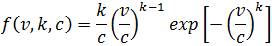
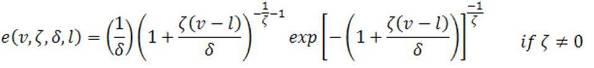
Where k is the shape parameter; c is the scale parameter; v is the wind speed; w is the mix parameter;  is the shape parameter of GEV distribution (dimensionless); δ is the scale parameter of GEV distribution (m/s); and l is the location parameter. During optimization process while performing load flow analysis, in order to account for wind DG power variation, at least hourly variations in wind power need to be considered which depend on average hourly wind speed. Hence 8760 number of wind states needs to be considered during optimization which is complex. To simplify analysis, the total 8760 wind states are represented by nine equivalent states (q). The probabilities (Pwg) of wind speed having speeds over different ranges (equivalent wind states) are computed using (3) and results are tabulated in Table 1.
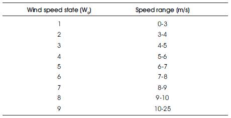
Table 1. Wind states and their corresponding speed ranges
Probability of each wind state is calculated by
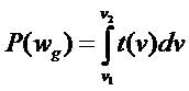
Where v1 and v2 are the speed limits of state wg. Wind turbine output power corresponding to each wind state is computed using the wind turbine power curve parameters as in (4). Average value of each state (vav) is utilized to calculate the output power of the turbine
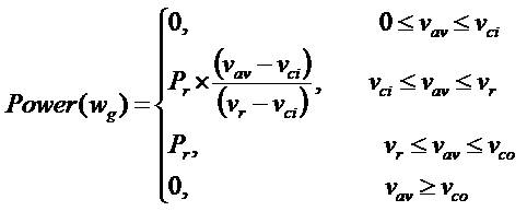
where vci, vr and vco are cut-in speed, rated speed and cut-off speed respectively. Capacity factor of a wind turbine is given by
To calculate annual energy loss by accounting for time varying load profile, multiple load flow simulations need to be done for different time intervals of a calendar year. For simplicity one hour is chosen as time step and hourly load profile data for 8760 hours in the year is used for load modeling. Hourly energy consumptions in each node are required for computation of energy losses. The selected IEEE 33 and 69-bus test feeders does not furnish hourly load data. Due to this reason, IEEE test system load data have been assumed as peak demands and demands for the rest of the year were found assuming the same load evolution as hourly load pattern of IEEE-RTS (Subcommittee P.M. 1979). So effectively there will be 8760 (=365*24) load states per annum.
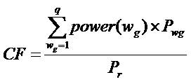
During optimization process, in order to compute actual annual energy loss, power flow analysis need to be performed incorporating time varying load profile characterized by 8760 load states which is complex and time consuming. Hence, to simplify analysis, the total 8760 load states are represented by ten equivalent states (r) with corresponding probabilities (PLg), using K-means clustering technique (Singh, C., Lago-Gonzales, A. 1989). Product of probability of a load state with annual number of hours gives the number of hours during which load is this particular state in a year. Ten equivalent load states are chosen which provides a fair trade-off between accuracy and fast numerical evaluation. Table 2 shows the computed ten equivalent load states with their corresponding probabilities. Load profile of a weekday and weekend in winter and summer seasons is shown in Figure1.
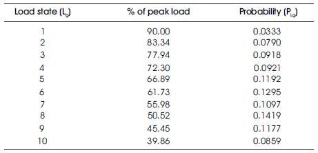
Table 2. Load states and their corresponding probabilities
Figure 1. Load profile of a weekday and weekend in winter and summer seasons
During optimization process in order to account for variations in wind power and system loads, combined states obtained by the product of equivalent load (r) and wind states (q) is used while doing power flow anlaysis. In this work it is assumed that there is no correlation between wind speed states and load states. Based on this assumption, the probability of any combination of wind based DG output and load is obtained by convolving the two probabilities as
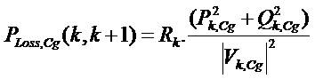
Power flows in a distribution system with variable DG output and time varying loads are computed by the following set of simplified recursive equations (Mekhamer et al., 2001) derived from the single-line diagram shown in Figure 2.

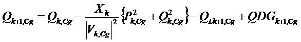
Where, Pk,Cg and Qk,Cg are the active and reactive powers flowing out of bus k during state Cg, PLk+1,Cg and QLk+1,Cg are the active and reactive load powers at bus k+1 during state Cg, PDGk+1,Cg and QDGk+1,Cg are the active and reactive powers injected by DG at (k+1)th bus during state Cg, Rk and Xk are the resistance and reactance of the line section between buses k and k +1.
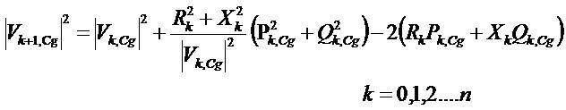
The power loss in the line section connecting buses k and k+1 during state Cg may be computed as
Total power loss of the feeder, PTLoss,Cg, may then be determined by summing up the losses of all line sections of the feeder, which is given as
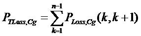
where n is total number of buses in the system.
The corresponding annual energy loss during state Cg is written as
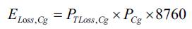
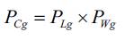
Where PCg is the probability of generation and load combination to be in state Cg and 8760 is the hours in the year.
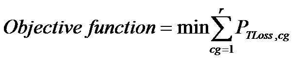
The objective function is formulated to minimize annual energy loss in distributed system considering all the states, which is given by
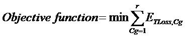
Where r is the number of combined generation and load states.
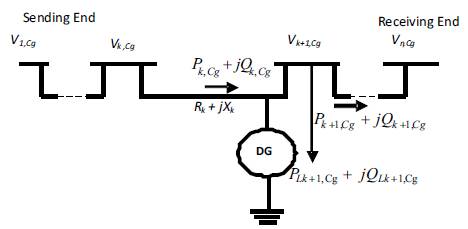
Figure 2. Single-line diagram of a main feeder
When constant load profile for system loads and constant DG output power are assumed while determining optimal DG sizes and locations, (7) to (11) are to be used in which the number of combined states cg is taken as one (cg = r = 1). Objective function is formulated to minimize active power losses is given by
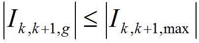
subjected to constraints specified in (13).
In this work sensitivity analysis is used to form a pool of top sensitive buses for DG placement. Instead of considering all the buses during the optimization process for finding locations, this pooled list is used which will reduce search space. This approach will improve the efficiency of the methodology in finding optimal locations.
Consider a line section consisting an impedance of Rk+jXk and a load of PLk,eff + jQLk,eff connected between k-1and k buses as shown in Figure 3.
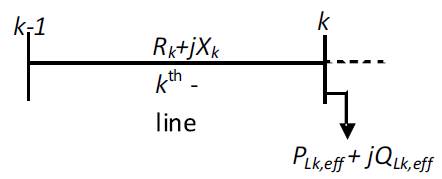
Figure 3. Electrical equivalent of a radial system
Voltage sensitivity index (Chakravorty M., Das D. 2001) is given by
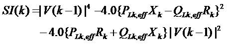
Where PLk,eff and QLk,eff are the total effective active and reactive powers supplied beyond bus k.
Voltage sensitivity index [VSI] for each bus is computed using (15) and a priority list of buses in ascending order is formed based on index values. Top 40 % buses in the list with minimum voltage stability indexes (prone to instability) are considered during DG location optimization.
This section discusses the steps involved in proposed and conventional methods.
The procedure to compute optimal locations and sizes of DG using proposed method considering uncertainty in wind power generation and time variant load profile is given as follows:
To compute actual energy loss with DG sizes and locations obtained, run load flow hour by hour for the entire year by changing hourly load as per time varying load profile and wind DG output obtained by (4) using average wind speed. Then power losses obtained for each hour are aggregated to obtain annual energy losses.
The procedure to compute optimal locations and sizes of DG using conventional method which assumes constant DG output and load profile is given as follows:
To compute actual energy loss with DG sizes and locations obtained, run load flow hour by hour for the entire year by changing hourly load as per time varying load profile and wind DG output obtained by (4) using average wind speed. Then power losses obtained for each hour are combined to obtain annual energy losses.
This section describes application of HS Algorithm for both proposed and conventional methods. Harmony Search Algorithm (HSA) is a meta-heuristic population search algorithm proposed by Geem, Z.W., Kim, J.H., Loganathan, G.V. (2001). HS algorithm parameters are Harmony Memory Size (HMS) or the number of solution vectors in the harmony memory; Harmony Memory Considering Rate (HMCR); Pitch Adjusting Rate (PAR); and Number of Improvisations (NI) or stopping criterion. The main steps of HSA are as follows:
Step 1: Initialize the algorithm parameters.
Step 2: Initialize the harmony memory.
Step 3: Improvise a new harmony.
Step 4: Update the harmony memory.
Step 5: Check the termination criterion.
Detailed description of these steps can be found in Geem et al., (2001) and Srinivasa et al., (2013).
For both proposed and conventional methods, application of HS Algorithm is similar with only difference being the objective function selection. In both methods, solution vector is designed to include both potential locations and sizes of DG. Suppose the number of DG units to be installed is N. Each solution vector has two parts where first part of solution vector has the DG sizes whose length is N and the second part corresponds to candidate buses which are chosen from the pooled list. Thus, the solution vector HV1 of length 2N for DG installation is formed as in (17):
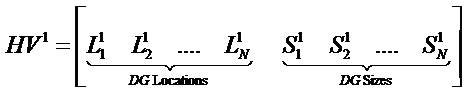
Where Sl1 Sl2 ... SlN are sizes of DG units installed at candidate buses Ll1 Ll2 ... LlN respectively.
Similarly, all other possible solution vectors are generated and the total Harmony Matrix generated randomly is shown in
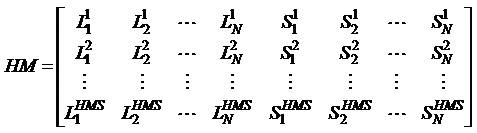
Objective function is evaluated for each solution vector of HM and HM vector is sorted in descending order based on their corresponding objective function values. The new solution vectors are updated as per steps 3 and 4. Using the new solution vectors, worst vectors of previous iteration whose objective function value is more will be replaced with new random vectors selected from the population that have lesser objective function values. This procedure is repeated until termination criteria are satisfied. Flow chart of the proposed method is shown in Figure 4.
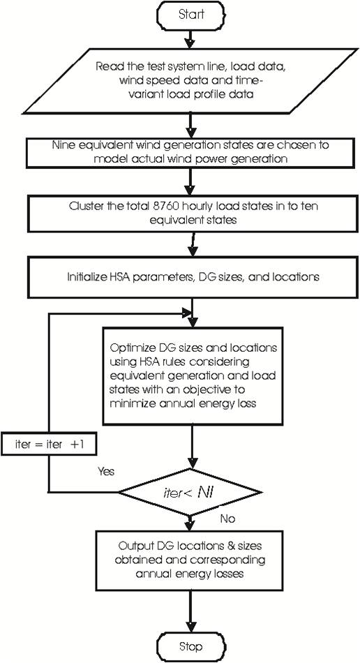
Figure 4. Flow chart for proposed method
In order to demonstrate the effectiveness of proposed method, it has been applied to two test systems consisting of 33 and 69 buses. For each test system, two scenarios are considered to evaluate the performance of proposed method and results obtained are compared with the results of conventional method. Both the methods are tested for 40% of maximum DG penetration. Parameters of HSA algorithm used for the simulation are HMS=50, HMCR=0.5, PAR=0.5, and NI =100.
Assumptions and constraints
Wind speed and turbine data:
Wind data: Wind data provided by National Data Buoy Center (http://www.ndbc.noaa.gov) for station 46012 (Half Moon Bay - 24NM South Southwest of San Francisco, CA) over a period of 3 years (2007-2009) is used to model wind power generation.
Wind turbine data:
Wind generation states with corresponding probabilities and percentage of rated power are shown in Table 3. Capacity factor of the chosen 100 kW turbine is computed using (5) which is equal to 0.5552. Predicted and observed wind frequencies of station 46012 are shown in Figure 5.
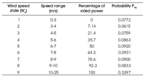
Table 3. Wind states and their corresponding percentage rated power
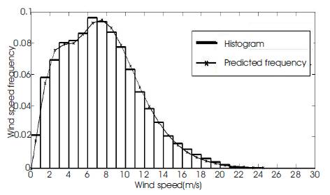
Figure 5. Predicted and observed wind frequencies of Station 46012
This system consists of 33 buses and the configuration, line and load data are taken from (Venkatesh, B., Rakesh Ranjan, Gooi, H. B. 2004), and the total active and reactive power loads on the system are 3715 kW and 2300 kVAR respectively. The annual energy loss assuming constant load profile is 1775.38 MWh, whereas the loss is 670.12 MWh considering time varying load profile for system loads.
The network is simulated using conventional and proposed methods considering DG installation at three locations and simulated results are presented in Table 4. Proposed method with 40 % DG penetration reduced energy losses from 670.12 Mwh to 437.04 Mwh by installing 700 kW, 200 kW and 800 kW at locations 15, 9 and 31 respectively. Conventional method reduced losses from 670.12 MWh to 449.60 MWh. Loss reduction achieved is less with conventional method since locations obtained are improper due to the assumption of constant load profile for system loads and fixed wind DG output. Hence, it is clear that conventional method is inadequate to compute optimal DG sizes and locations resulting in lesser percentage energy loss reduction.
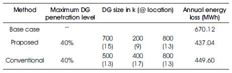
Table 4. Results of 33-bus System
69-bus radial distribution system is a large scale system with total system loads of 3802.19 kW and 2694.06 kVAR. The configuration, line and load data are taken from Savier, J. S., Das, D. (2007). The annual energy loss assuming constant load profile is 1970.82 MWh, whereas the loss is 737.72 MWh considering time varying load profile for system loads without DG. The base case voltage sensitivity indexes of top 40% sensitive buses are arranged in descending order as shown in Table 5 which are used for location optimzation. Results obtained with both the methods are presented in Table 6. With 40 % DG penetration, the percentage energy loss reductions are found to be 39.60 and 34.63 using conventional and proposed methods respectively. Percentage loss reduction with proposed method is better than conventional method. Above analysis shows that energy loss reduction achieved using proposed method is the highest, which demonstrates its superiority over the conventional method.
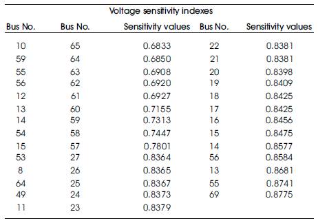
Table 5. Sensitivity Values of 69-bus System
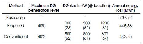
Table 6. Results of 69-bus System
In this paper, a new method that employs Harmony Search algorithm is proposed to install multiple wind based DG units optimally in distributed system with an objective of minimizing annual energy loss considering variability in generation and system load profile. In conventional methods optimal DG sizes were found assuming constant load profile and fixed DG output generation. It is shown that considering time-varying load profile and uncertainty in generation significantly affects the optimal location of DGs. Based on the results, it is observed that energy loss reduction with proposed method are high.