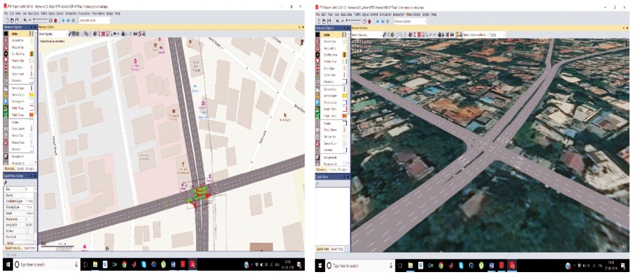
Figure 1. Intersections in 2D &3D
The study aims at developing a micro-simulation model for signalized intersection to reduce the travel time by improving the signal program. The data collection includes Classified Turning Volume count at the Intersection, Geometry of the Intersection, Signal Timing and Phasing and Delay and Travel Time across the intersection. The model is developed in PTV (VISSIM) “Verkehr In Städten - SIMulationsmodell” and is calibrated using Genetic Algorithm (GA) through the Component Object Model (COM), Application Programming Interface (API) enabled through MATLAB, also by manual systematic adjustments of parameters, which is then validated with a different dataset with a Mean Absolute Percentage Error (MAPE) within the limit of 15%. Results from the Simulation after signal program optimization indicated a reduction in the travel time upto 25% to the users.
Traffic intersections are complex locations because vehicles moving in different direction want to occupy same space at the same time. In addition, the pedestrians also seek same space for crossing. Drivers have to make split second decision at an intersections by considering his route, intersections geometry, speed and direction of other vehicles etc. A small error in judgment can cause severe accidents. It also causes delay which depends on type, geometry and type of control. Overall, traffic flow depends on the performance of the intersections. It also aspects the capacity of the road. Therefore, from both the accident and performance perspective, the study of intersections is very important for the traffic engineers especially in the urban scenario (Mathew & Krishna Rao, 2007).
Signalized intersections are subjected to active control i.e., time sharing and unsignalized are characterized by passive or no control, i.e. space sharing (Mathew & Krishna Rao, 2007). An unsignalized 4-Legged intersections having two-way traffic movement have 32 conflict points of which 16 are major and 8 are minor conflict points whereas if one of the two roads are declared one way, the conflicts drop down to just 11 with major and minor conflicts of 7 and 4 respectively. Khanna et al. (2014), said that further by signalization of such intersections we can totally eliminate the conflicts or leave a residue of 1 or 2 minor conflicts for the free left-turning merging moments.
Bengaluru metropolis experienced explosive development in the recent years which the planners had not foreseen due to which the infrastructure suffers to meet the unsatiating traffic demand. PTV VISSIM is a microscopic time step and behavior-based simulation model developed to model urban traffic (Dowling et al., 2004; Fang & Elefteriadu, 2005; Manjunatha et al., 2013). The program can analyze traffic and transit operations under constraints such as lane configuration, traffic composition, traffic signals, transit stops and so forth, thus making it a useful tool for the evaluation of various alternatives based on transportation engineering and to plan measures of effectiveness (Ashalatha et al., 2018).
The present study involves modeling a typical urban signalized intersections in VISSIM (“Verkehr In Städten- SIMulationsmodell”) Doina and Chin (2007), which is a popular microsimulation modelling tool used to analyse traffic. The primary objective for this study is to develop, calibrate and validate intersection model for heterogeneous traffic conditions. Subsequently, experimental the signal timing and phasing is recorded to correspond the effect on the intersection performance.
The initiation towards the primary objective of developing a well calibrated and validated model of the intersection is to gather the necessary data. The next step is to represent the intersection geometry in the network editor of VISSIM. The vehicular characteristics (static & dynamic) are defined, traffic flow, composition and turning proportions are collected, extracted, prepared and input into the software, signal timing and phasing is programmed into the software similar to the field. The data collection points, queuing counters added in the network, act as stations for measuring queue length and gather other necessary results from the simulation. Subsequently, the parameters significantly influencing the simulation have to be identified, therefore a sensitivity analysis is carried out [Mathew & Radhakrishnan, 2010; Siddharth & Ramadurai, 2013]. Then the model is calibrated using Genetic Algorithm enabled by MATLAB optimization toolbox and COM interface of VISSIM. Also, by trial and error method of systematic manual adjustment of attributes, the calibrated models are then validated with a data set from another time. Finally, the signal timing is rescaled and its effect on the travel times across the intersections and queue length development is recorded.
Shoolay circle is one of the signalized junctions present on Richmond road. It is one of the heavily congested roads in Bengaluru. Due to number of schools and shopping malls present in this area the traffic volume increases to a very great extent during peak hour of weekdays and weekends.
Classified turning volume count across the intersection during morning and evening peak hours of 8:30 A.M to 10:30 A.M and 5:30 P.M to 8:30 P.M respectively was carried out using video graphy technique on Monday and Sunday to represent the weekday and weekend traffic. Data extraction was done to determine the flow in vehicles per hour at every fifteen-minute interval, and the vehicular composition was synchronously determined. The signal timing and phasing were also extracted from the video.
The delay and travel times across the intersection were determined by the floating car method for an average of 3 trials. This was done simultaneously while recording. Gradient of links were measured using GPS.
Modelling of Traffic in general can be fragmented into the tangible physical part and the intangible dynamic behaviour part. The modelling of the first fragment in VISSIM requires intersections geometry (approach width, lane numbers. bus stop attributes and other roadside features and gradients), Vehicular characteristics (dimensions, speed, acceleration and deceleration distributions), Traffic Inputs (flow, compositions, turning volumes etc.), Signal timing and phasing plan. Modelling the driving behaviours i.e., the second fragment is carried out by modifications to the attributes behaviour models already built-in VISSIM.
VISSIM offers in-built map providers such as Bing maps and Open street map (Mapnik) in which intersections are located and thus providing a background to build geometry of the intersection. Alternatively satellite images can be imported into the software, which is scaled and used for the same purpose. The representation of nonstandard lane width is a significant criterion for accurate simulation of urban intersection, but doing so while modelling is a tricky affair, this is done so by distributing available road width to the number of lanes equally i.e., A road width of 9m is adopted as 3 lanes of 3 meters or 2 lanes for 4.5m suitably. The perks of this methods is well described in the work of Mathew and Radhakrishnan (2010). The gradient has an effect on the acceleration and deceleration of vehicles measured from GPS, therefore a measured gradient of +2.54 to -2.77 for Richmond road, 0.74 to 0.65 for Hosur and Brigade road are found respectively. This gradient is not updated in the GUI due to the limitations of software but is accounted for during simulations. Subsequently, routing decisions are defined and the corresponding proportion of turning traffic is assigned. Signal heads and travel time sections are marked. The geometric representation of the intersections is show in 2D and 3D with both map services as shown in Figure1.
Figure 1. Intersections in 2D &3D
Another major aspect in modelling are vehicles, such as defining the static characteristics like length and width, the dynamic characteristics like speed, acceleration, deceleration distributions for the various types of vehicles. Such data specific to our intersection warrants an exhaustive study of its own, which is beyond the scope of this study, therefore these data are adopted from similar studies from the past (Fang & Elefteriadou, 2005).
VISSIM provides a library of various types of standard vehicular models, unfortunately, the autorickshaw (threewheeler) isn't one of the models included in the library, which owns a significant composition in our traffic stream to be simply disregarded. As a work around for this problem, we utilized a base model of a car dimensionally nearest to the auto's and incorporate the three wheelers dimension into it, if not visually this method is computationally verified to work as intended. The details of traffic, vehicle dimensions and approach widths are indicated in Table1.
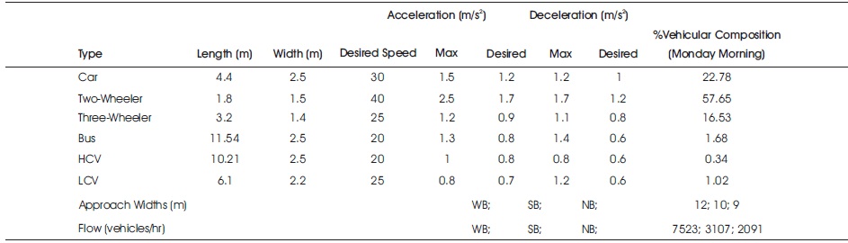
Table 1. Intersection Geometry, Vehicular Characteristics and Traffic Flow at Intersections
VISSIM incorporates four driving behaviour models namely Car following model, Lateral model, Lane change model and Signal control model to logically replicate the real world traffic behaviour. By default these models are tuned to homogeneous lane disciplined traffic, but to simulate heterogeneous non-lane-based traffic conditions prevalent in developing countries like India, the attributes of these behaviour models have to be modified. One such main change to be made is to the lateral behaviour, by change the desired position at free flow selection from “middle” to “any”, Overtaking on left side and right-side is allowed, similarly the various model attributes are changed according to match the intersection understudy.
The signal program for this intersection exists in two phases i.e., signal groups. The first group facilitates all three turning moments for the Richmond road (One-way) (Westbound), the second group allows through moments for the cross roads (Northbound & Southbound). There is a free left turn for S-W traffic flow. The signal program and Phase diagram are indicated in Figures 2 and 3. The signal heads are to be placed on the respective lanes and the corresponding signal group is assigned to them. It is important to exercise caution in placing the signal head on links while modelling because placing them on the connectors will make the vehicles disobey the signal. However, this interaction in the software can be utilized to our advantage to model the free left turning vehicles, which otherwise would pose a modelling challenge as there is no option to differentiate the traffic based independent lane groups and assignment of signal heads. In our intersection the signal head is placed further ahead of the left turning connector at the northbound approach to simulate the free left turn movement. Signal phase is synonymous with signal group, which is popularly used in various countries. The terminology adopted in the software with this reference is henceforth, used in this study.
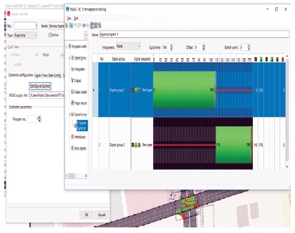
Figure 2. Signal Control Programmed in VISSIM

Figure 3. Intersection Turning Moments and Signal Phasing
Prerequisite for calibration is to conduct a sensitivity analysis by manual comparison of field and simulated delay to identify the attributes of the various behavior models which are having significant impact, and the range of values which these attributes exhibit sensitivity are also determined to reduce the overall computation effort out [Mathew & Radhakrishnan, (2010); Siddharth & Ramadurai, (2013). Calibration of the model is one of the most significant and challenging step as it makes or breaks the model. The efficacy of the model is hugely dependent on this step. Calibration is basically the process of adjusting the model parameters to minimize the discrepancy between the field measurements and simulation values. In this study, an attempt is made on automated calibration using Genetic Algorithm solver in MATLAB and a manual approach to systematically adjust the parameters to minimize the absolute difference between the delay at field and delay from the simulation. The mathematical formulation of the objective is indicated by Equation1.
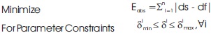
Where, ds = the intersection delay obtained from this simulation model;
df= the field delay measured;
δ'min & δ'max = lower and upper bounds for the ith parameter;
j = Simulation run with random seed increment.
The parameters considered in this study and their ranges are indicated in Table 2.
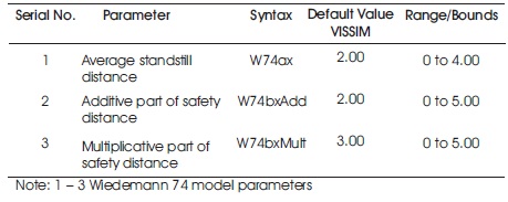
Table 2. Driving Behavior Parameters in VISSIM (selected for calibration of this model)
The Component Object Model(COM) interface enables the access to VISSIM through MATLAB, Equation 1 is the input argument for evaluation of fitness of the population, the other two inputs required to run the solver are number of variables(nvars), which is 3 in our case and their constraints i.e., their upper and lower boundaries are indicated in Table 2. Thus for defining the optimization problem, simply put, GA searches for the optimum set of the three calibration parameters, which presents us with the minimum error. The single crossover rate is set to 80%, Uniform mutation rate is specified at 1%, Elitism is activated to carry forward the fittest members of the population, A script file in MATLAB is written to co-ordinate the working of VISSIM with the algorithm. Thus, iterations are performed till convergence, the output from the GA optimizes the set, though it does not guarantee a global minimum out (Mathew & Radhakrishnan, 2010), i.e., there could exist another set of parameters which could yield a lower error.
The need for such a heuristic process, is that it substantially reduces tedious manual effort of systematically changing the parameters, also the probability of landing on a set, in which local minimum is reduced, thereby maximizing the performance of the model, which is not far from the representation of the field conditions and results.
The Results of calibration with GA data of one approach is indicated in Table 3. Note: However, with these set of parameters, the simulation returns a warning “Vehicle input 1 could not be finished completely remain: 850 vehicles”, since the number of vehicles is very high this cannot be disregarded to be trivial as in the case documented in memorandum by Ray Shank, (2014) for minor remains such as 4 vehicles, thereby casting ambiguity, necessitating further investigation and improvement to the code.

Table 3. Results of Calibration with GA with Data of One Approach (Approach 1) Using Wiedemann 74 Model
In this method, the model is initially simulated using default parameters, if the Mean Absolute Percentage Error (MAPE) between the observed and simulated delays is high, then the parameters are changed one by one keeping the others constant such that the MAPE is reduced. Table 4. illustrates and presents the results of such manual calibration procedure. Finally, the parameters with least MAPE value are considered as calibrated values, the final calibrated values are shown in Table 5.
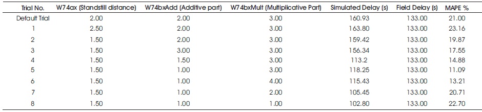
Table 4. Trials for Manual Calibration with Combination of Attributes
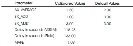
Table 5. Final Calibration Attribute Values Adopted
These values are acceptable and are with in the limits of 15% proposed by Dowling et al. (2004) and accepted by similar studies of Ashalatha et al. (2018), Mathew and Radhakrishnan (2010), Arroju et al. (2015), Siddhart and Ramadurai (2013). Therefore, the model can be confidently used.
Note: As discussed in previous section these parametric values successfully complete the vehicle inputs into the network and are henceforth adopted.
This model is validated for the selected calibrated parameters with a different data set collected during evening peak for this purpose. Validation results are within 15%, which is in acceptable range and confirm with the results recorded in similar studies) (Mathew & Radhakrishnan, 2010) Dowling et al. (2004). The results are presented in Table 6.
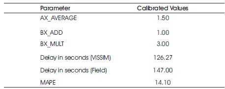
Table 6. Results of Validation with Evening Data
The secondary objective is optimization of signal program, the maximum and average queue lengths are developed and Travel Times for approaches 1 and 2 were obtained from the simulation model. Westbound approach (1) and Northbound approach (2) are only considered because Southbound approach (3) has higher road width than approach 2 (from geometry survey).
The model was simulated for 4200 seconds with a warm-up period of 600 seconds, allowing the road network to saturate. A total of 5 simulations were run with a random seed increment of 12 to eliminate the effect of stochasticity. The data was collected between 600 – 4200 seconds of the simulation at an interval of 600 seconds. The aggregate values of travel times and queue lengths developed are recorded. The results along with the existing signal program timing is shown in Table 7.
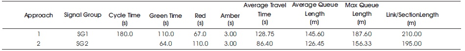
Table 7. Simulation Results with Exiting Signal Timing and Phasing
If the queue length grows beyond the link length, the cross flow of traffic is negatively affected. Additionally it may cause rear end blocking of the upstream intersections or cross roads, therefore queue length is restricted to be within the Link/Section length. Therefore the limiting queue length for Westbound-approach (1) is considered as 200 m as there is an intersection at 220 m from this approach and for Northbound-approach (2) it is considered as 185 m as there is an active crossroad at a distance of 201 m.
For the optimization exercise, the share of green time of signal group 1(SG1) is gradually increased by five seconds, which consequentily reduces the green time of signal group2 (Sg2). The results are recorded in Tables 8 and 9 for approach 1and approach 2 respectively.
From the output, we can infer that the signal program is optimized up to shift of 20 seconds in green time after which the queue length of approach 2 exceeds the critical limit.
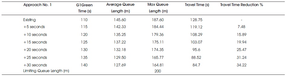
Table 8. Results of Green Time Variation For West Bound Approach (1)

Table 9. Green Time Variation for Northbound Approach (2)
The primary objective of developing a well calibrated and validated simulation model of signalized intersection was achieved with a manual calibration error of 11.09% and a validation error of 14.10%. The automated calibration using GA requires further troubleshooting for valid consideration.
The secondary objective is to optimize the signal program to improve the overall performance of the intersection in terms of the travel time presented below,
Therefore, 20s green time shift is optimum as it has a 25.47% reduction in travel time for approach 1 and 12.24% increase in travel time for approach 2., also satisfying the maximum queue length criteria with 182.33m.
The authors are thankful to RV College of Engineering for providing the necessary facilities for carrying out this study, and Professor K. Parthan, Asst. Professor, Dept. of Civil Engg., BMSCE for supporting in the work.