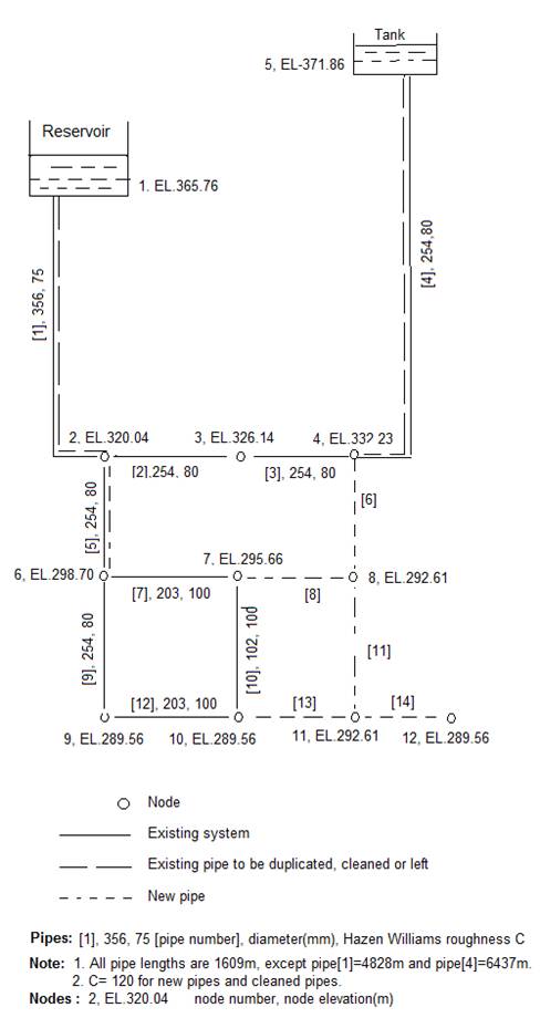
Figure 1. Layout of Gessler (1985) pipe network
A good water distribution system (WDS) continues to deliver water at all nodes of pipe network to fulfill various water pressure and demand conditions. In this paper, the authors used Genetic Algorithms (GA), a methodology for optimizing pipe networks. A computational code has been developed using Matlab software for optimization of pipe network. To ensure the validity of the code developed, it was tested with the Gessler (1985) pipe network design. This tested code can be further used for design and analysis of pipe network.
Water Distribution system (WDS) is a network of pipes,tanks, pumps and other accessories grouped together to transport the fluid from one place to other. The construction, maintenance and operation of this network are expensive. Design and analysis of pipe networks is a complicated problem, particularly if the network consists of different sizes of pipes. In recent economic scenario we expect the highest return of each single penny spent. To meet this objective, design engineers opt for optimization of pipe network. This is achieved by selection of commercially available pipes that fulfil the flow demand and pressure head at each node.
The aim of WDS optimization is to find the least cost solution which satisfies all hydraulic constraints at different nodes of that network. Various approaches such as linear, nonlinear, dynamic, evolutionary, integer and mixed integer programming were adopted by the researchers for optimization.
Alperovits and Shamir (1977), Quindry et al. (1981) presented a linear programming (LP) method for optimization of WDS. Stephenson (1984) presented simplex method for optimization of tree network. Morgan and Goulter (1985) presented heuristic LP approach for WDS to obtain least cost design value.
In least cost design of water distribution system (WDS), the objective function with some constraints is a nonlinear function. Many researchers came forward with non-linear programming packages. Gupta et al. (1993) developed the software package WATDIS. Lansey and Mays (1989) presented Generalized Reduced Gradient (GRG) model for least cost design of water distribution system. Fujiwara and Khang (1990) further presented two stage optimization technique.
Samani and Mottaghi (2006) presented binary linear programming (BLP) model for optimization of WDS. In this model, objective function and constrains are linearized.
Researchers have applied evolutionary optimization technique over gradient based technique to overcome the limitations of traditional optimization method of WDS. Evolution Algorithms (EA) are able to provide near global optimum solution and have less possibility of being trapped in local optima. Various EA have been developed for optimization of WDS design. These were first introduced as genetic algorithm by Simpson et al. (1994).
Genetic Algorithm (GA) is the most frequently used Evolution Algorithms (EA) due to their easy implementation and better search ability. An improved GA was proposed by Dandy et al. (1996) for WDS optimization in which, gray coding was introduced. Vairavamoorthy and Ali (2000) used integer coding for GA. Deb (2000) introduced tournament selection algorithm to handle constraints. Wu et al. (2001) presented fast messy genetic algorithm (mGA). Nicklow et al. (2010) presented a GA that is flexible and a powerful technique to solve complex WDS networks. Zheng et al. (2011e) applied on various case studies with different decision variables ranging from 21 to 1050 and concluded that GA is current best known technique of finding global optimum solution.
To tackle the minimum head constraint and minimum discharge constraint, penalty cost is added to the actual cost of the network.
A good Water Distribution System (WDS) is to deliver water at all nodes of pipe network to fulfill various water pressure and demand conditions. Using Genetic Algorithm as optimization tool, a computational code has been developed by means of Matlab software for optimization of pipe network. To validate the mathematical model developed, it has been tested with Gessler (1985) pipe network as shown in Figure1.
Figure 1. Layout of Gessler (1985) pipe network
The optimized data is compared with Simpson (1994) optimization design, the known solution given in literature which used the same pipe network. All other data such as objective function, cost function of pipe, pipe sizes, and cost of the pipe are taken from Simpson (1994).
Network shows solid lines, representing the existing system, dashed lines depicting the new pipes and elevations, pipe lengths, diameters and Hazen-Williams (C) coefficients are also shown. The network has following features.
1. All pipes are 1609m long, except pipe [1] =4828m and pipe [4] =6437m.
2. The Network must fulfill these conditions.
3. C=120 for new pipes and cleaned pipes.
4. Available pipe sizes and associated cost (for Case Study) is mentioned in Table 1.
5. A value of K = $70,000/m is chosen for the penalty function multiplier.
6. Demand Pattern and Associated Minimum Pressure for Network is given in Table 2.
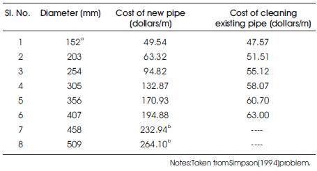
Table 1. Available Pipe Sizes and Associated Costs for Case Study Network
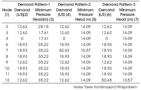
Table 2. Demand Pattern and Associated Minimum Pressure for Network
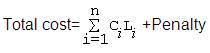
1. The objective function of the pipe network is to minimize the total cost. Neglecting the other factors, it is assumed that actual cost of the network solely depends upon pipe geometry (commercially available pipe). To tackle the minimum head constraint and minimum discharge constraint, penalty cost is added to the actual cost of the network.
Minimum cost (z)

Here, C1, C2 and C3 are shown in Table 3, L represent length of the pipe, J represent five new pipes [6], [8], [11], [13] and [14]. Similarly, k represents pipe [4] and [5].
2. The penalty cost is superimposed on top of the actual cost of the network in such a way that it will discourage the search in the infeasible direction.

Subjected to:
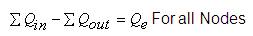
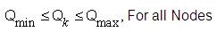
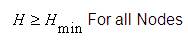
Where Qin =flow into the junction; Qout =flow out of the in out junction and Qe external inflow or demand at the junction node, n is the number of pipes in network, k represents node number, Q and H represents the discharge and Pressure head required at nodes respectively. L represents length of the pipe and C represents cost function of the pipe as shown in Table 3.
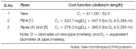
Table 3. Fitted Cost Functions for Nonlinear Optimization Model Pipes
3.The GA assigns a penalty cost for each case, if a network doesnot fulfil the minimum pressure constraints. The maximum pressure deficit is multiplied by a penalty factor (e.g., K = $70,000/m of head). The penalty multiplier is a quantity of the assessment per meter recognized to pressure heads below the allowable minimum pressure head. K=$70,000/m, taken from Simpson (1994) problem.
4. In the GA formulation for test problem, eight variables (five new pipes and three existing pipes), each represented by a three-bit binary substring were selected representing eight possible alternatives as shown in Table 4.
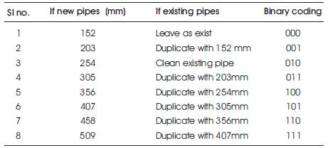
Table 4. Options for each decision variables
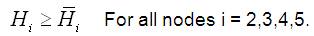
5.There were totally 110 constraints for three demand patterns as shown in Table 2.
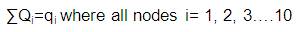
Where Qj is the discharge in pipe number j meeting at node i and qi is nodal withdrawal at node I.
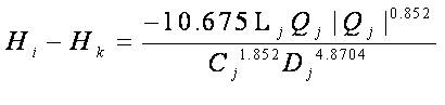
Where Lj =Length of the pipe, Dj = Discharge inflow in pipe and Cj =Hazen Williams coefficient for pipe j.
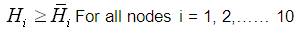
These three items give 34 constraints per demand pattern as given in Table 2.
There were a total of 110 constraints (i.e., 3x34 + 8 =110) for the given problem.
Pipe network optimization is achieved by using Genetic Algorithm comprising reproduction, crossover and mutation. A software program has been developed on MATLAB for getting optimal or near optimal solution for this case study.
In Table 5, the population size (50), crossover point (single), and mutation rate (0.05) are kept constant and number of iterations and crossover percentage goes on changing. It is observed from convergence table of Figure 2 and Table 5 that, fitness values are very close at crossover percentage of 80% and 100%. Similarly, the fitness value at iteration rate 300 and 500 are very close. So the authors selected crossover percentage as 80% and number of iteration as 300 for further convergence of fitness value. Convergence Table 1to 3 show the variation of fitness values with different parameters of GA.
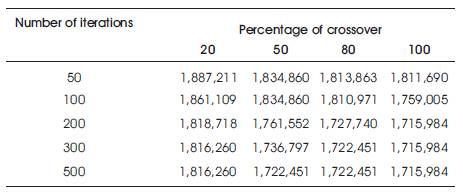
Table 5. Fitness Value (Total cost of network in Dollars) Vs Percentage of Cross over
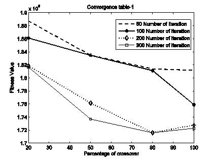
Figure 2. Percentage of Crossover Vs Fitness Value
In Table 6, the number of iteration (300), crossover point (single), and percentage of crossover (80%) are kept constant and mutation rate as well as population size goes on changing. It is observed from Table 6 that, fitness value of population size at 300 and 500 are very close. Similarly, the fitness value at different mutation rates are very close. So, the population size is selected as 300 and mutation rate as 0.05 for further convergence of fitness value (Figure 3).
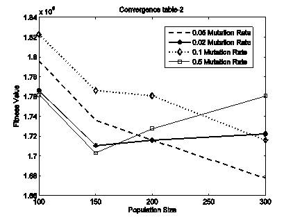
Figure 3. Population Size Vs Fitness Value
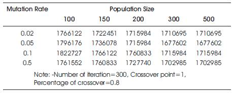
Table 6. Variation of Fitness Value (Total cost of network in Dollars) at different Mutation
In Table 7, the fitness values are very close at one point, two point and three point crossover as shown in convergence Table of Figure 4. Here the single crossover point is taken.
However, the authors opt for Population size (300), percentage of crossover (80%), number of iteration (300), mutation rate (0.05) and single point crossover to find the optimum value (minimum value) of network cost. The best nine solutions (Total cost of network in Dollars) that satisfy all Constraints are given in Table 8. The optimum value of Gessler (1985) pipe network is 1,467,008Dollars which is much lower than earlier calculated fitness value in literature.
The best results (minimum total cost of network) from Table 8 is shown graphically in Figure 5.
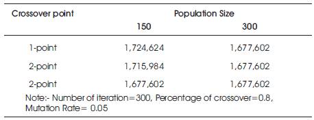
Table 7. Fitness Value (Total Head Lossin Dollars) vs different Crossover point
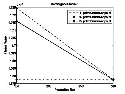
Figure 4. Population Size Vs Fitness Value
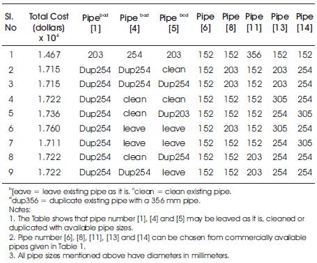
Table 8. Best nine solutions that Satisfy Pressure and Demand Constraints
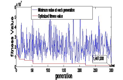
Figure 5. Generation Vs Fitness value (Best Cost Results)
The Genetic algorithm deals with the eight decision variables in the Gesseler(1985) pipe network. Each variable is represented by a three bit binary substring. The three bit represents eight possible alternatives for either new pipes, duplicated pipes or cleaning of an existing pipe (Table 4).A 24-bit binary string represents the network to be optimized.
The fact that the problems considered do not have pumping facilities is simply because these problems were taken from literature. The authors developed a MATLAB computer program of a standard three operator GA. Optimum cost of network is shown in Table 8.
The mathematical model developed is applied for optimum design of another pipe network (Case Study) as shown in Figure 6, the demand pattern and associated minimum pressure are given in Table 9. This network has five number of pipes and five number of nodes as well. The discharge Q2 , Q3 , Q4 and Q5 are flowing through pipe number 1,2,3,4 and 5 respectively. Similarly, q2 , q3 , q4 and q5 are the nodal withdrawal of water from nodes 2, 3, 4 and 5 respectively. Other parameters such as pipe sizes are the same as in Simpson (1994) pipe network.
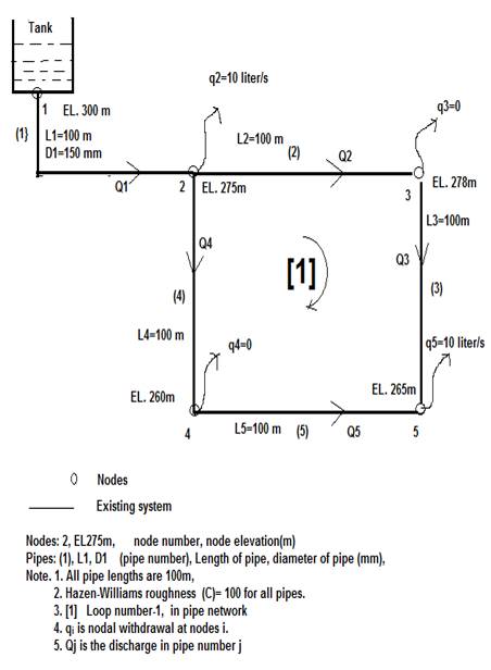
Figure 6. New pipe network for case study

Table 9. Demand Pattern and Associated Minimum Pressure for Network
To implement the GA, following parameters has been taken.
1. All pipes in given network can be chosen from commercially available pipes. The objective function (Cost functions in dollar) is taken from Simpson (1994)

2. There are four demand constraints and four pressure constraints in this network. (Total number of constraints are eight.)
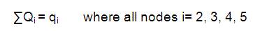
Where Qj is the discharge in pipe number j meeting at node i and qi is nodal withdrawal at node i.
3. A value of K = $10 is chosen for the penalty function multiplier from Deb(2000).
4. Other parameters are same as in Simpson (1994) pipe network.
5. Population size = 300, probability of crossover= 0.8, probability of mutation=0.05and single point crossover are taken to find the optimum value (minimum value) of network. The best three solutions (Total cost of network in Dollars) that satisfy all Constraints are given in Table10. The fitness value vs population generation is shown in Figure 7.

Figure 7. Fitness Value (Best cost results) in dollars Vs Population Generation
The Genetic algorithm deals with the five decision variables in the new pipe network (Figure 6). Each variable is represented by a three bit binary substring. The three bit represents eight possible alternatives for commercially available new pipes (Table 4, 2nd column).A 15-bit binary string represent the network to be optimized.
The authors developed a MATLAB computer program of a standard three operator GA. Optimum cost of network is shown in Table 10.
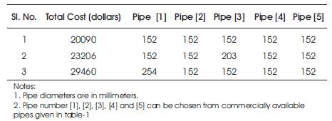
Table 10. Best results (Minimum total cost of network in Dollars)
GA algorithms has shown efficiency and effectiveness.
The GA finds the minimum cost configuration of Gesseler Pipe network. The authors establish that the genetic algorithm method using the standard three operators comprising reproduction, crossover, and mutation, is particularly effective in finding global optimal or near optimal solutions for the water pipe network.
The genetic algorithm technique is appropriate to discrete variables such as selection of commercially available pipe sizes and hydraulic constraints. The genetic algorithm technique is in its research stage, and further developments can improve the search methods for large size practical problems.