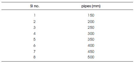
Table 1. Details of Commercially Available Pipes
Liquid and solid are two phase flows, stated to as slurries. Slurry particle less than 40 μm (fine particles) in turbulent flow behave in a homogeneous manner. They are referred to as non-setting slurry. The particles’ concentrations are almost similar across the cross section of pipe. The characteristics of slurry such as unsteady flow rate, complicated ingredients, high concentration and viscosity of liquid carrier are subjected to pipeline blockage and high energy consumption. The pressure drop is a key parameter in the design of slurry pipelines, as it delivers evidence on the power required to continue a flow rate above the critical deposition velocity. As the pressure drop in pipeline is directly proportional to the energy consumption, to minimize the pumping cost of slurry, the pressure drop must be minimum. This paper presents an overview on the head losses in pipeline for slurry flows. The minimization of the head loss is considered as the objective function. Genetic algorithm is used as the optimization technique and code is developed in MATLAB.
Due to low operating and maintenance cost, slurry pipelines are commonly used in pharmaceuticals, mining, and chemical industry for long distance transport of solids to processing unit. Countless struggle has been made towards the growth of reliable models for the pressure drop and solids concentration dispersal in slurry pipelines. Durand and Condolios (1952) were some of the first to mature empirical models. Wasp et al. (1977) upgraded their calculation by integrating the effect of varying size particles. Wilson (1976) develop a two-layer model where each layer has an even concentration and averaged velocity, which was later amended by a three layer model offered by Doron et al. (1987). Amongst these, two layer model of Gillies et al. (1991) is often used in the literature for predicting the pressure drop in slurry pipelines.
Coal water slurry pipeline, iron ore transportation, mineral concentrate pipeline, sand removal and fly ash disposal are major applications of slurry transportation. Wilson (2005); Shen (2010), mentioned the advantages of slurry pipelines over other transportation means. A large number of these industrial suspensions do not obey Newton's law of viscosity and therefore referred to as non- Newtonian suspensions.
The hydraulic transportation of solids in pipelines are connecting locations often distance more than 100 kilometer apart. In this process, energy consumption is very high, Jacobs(1991).The aim of the optimization problem in the study is to minimize the pumping cost of slurry. An attempt has been made in the present study to modify Durand and Stepanoff, (1969) model for head loss in the pipe by Genetic algorithm (GA). The GA optimization tool can increase the probability of finding the global maximum or minimum.
In this paper, Genetic Algorithm (GA) is adopted as optimization tool. Genetic Algorithm from its inception, has successfully solved the discontinuous and non differential function optimization problem which traditional numerical method failed to solve. The energy consumption of slurry transportation may be achieved by minimizing the head loss in a pipe network.
For our case study, a pipe network is considered which contains one kilometer pumping main pipeline which in turn carries a slurry of average sediment particle size of 40 μm with mass densities of particles and fluid ratio as 2.5. The details of commercially available pipe size and the average roughness height of pipe materials are given in Tables 1 and 2.
Table 1. Details of Commercially Available Pipes
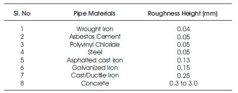
Table 2. Average Roughness Heights
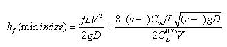
Durand and Stepanoff (1969), gave the following equation for head loss for flow of fluid in a pipe with heterogeneous suspension of sediment particles
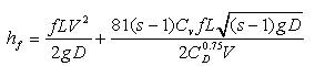
Where s=ratio of mass (densities of particle and fluid, Cv =Volumetric concentration, CD = Drag coefficient of particle, and f = friction factor of sediment fluid, D=diameter of pipe, L is the length of the pipe, g is acceleration due to gravity.
Swamee (1993) gave the following equation for friction factor (t) valid in the laminar flow, turbulent flow and transition in between them.
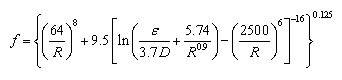
Where the roughness height of the pipe material in meter is ε, R is the Reynolds number given by,

Where V is the Average velocity of flow m/s, v is the kinematic viscosity of fluid in the pipe.
The kinematics viscosity (V) of fluid can be obtained using the equation given by Swamee (2004),
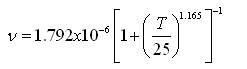
Where T is the water temperature in °C
For spherical particle of diameter d, Swamee and Ojha (1991) gave the following equation for CD .
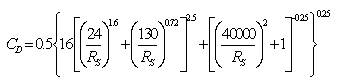
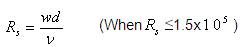
Where Rs =Sediment particle Reynolds number given by
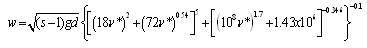
According to Swamee and Ojha, (1991), the fall velocity (w) is given by
In the GA formulation for test problem, five variables namely Temperature Variable (T), Average Velocity Variables (V), Volumetric Concentration (Cv ), Diameter of Pipes (D), and Roughness height (€) were each represented by a three-bit binary substring, which were selected representing eight possible alternatives as shown in Table 3.
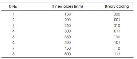
Table 3. Details of Commercially Available Pipes with Binary Coding in GA
The objective function of this given network is to find the minimum head loss in pipe,
The following parameters have been taken. Population size=100 to 300, probability of crossover= 0.2 to 1.0, probability of mutation=0.01 to 0.05, Dimension=5, string length=3.
A software programming has been developed on MATLAB for getting optimal or near optimal solution for this case study.
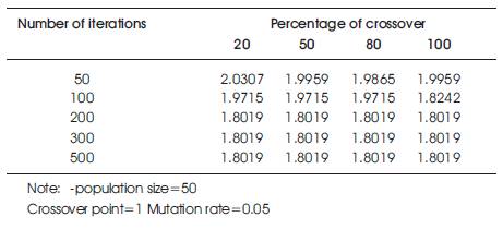
Table 4. Total Head Loss in meter
In Table 4, the population size (50), crossover point (single), and mutation rate (0.05) are kept constant and number of iterations and crossover point changes. It is observed that fitness value at higher crossover and at higher iteration rate are very close. So we selected crossover as 80% and number of iterations as 300 for further convergence of fitness value.
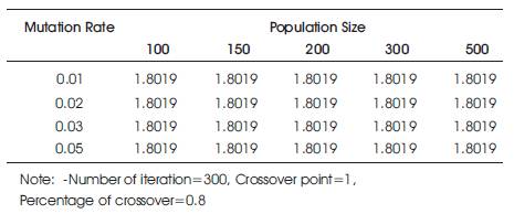
Table 5. Total cost of network in Dollars
In the following Table 5, the number of iterations (300), crossover point (single), and percentage of crossover (80%) are kept constant and mutation rate as well as population size goes on changing. It is observed that fitness value at population size at 300 and 500 are very close. Similarly, the fitness value at different mutation rates is very close. So we selected population size as 300 and mutation rate as 0.05 for further convergence of fitness value. Figure 1 to Figure 4 show the variation of fitness values with different parameters of GA.
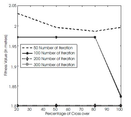
Figure 1. Fitness Value (Total Head Loss) vs Percentage of Cross over
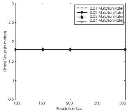
Figure 2. Variation of Fitness Value (Total Cost) with Population Size at different Mutation Value
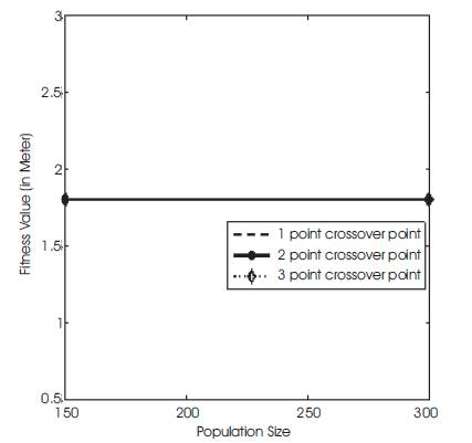
Figure 3. Variation of Fitness Value (Total Cost) with Population Size at different Cross Over Value
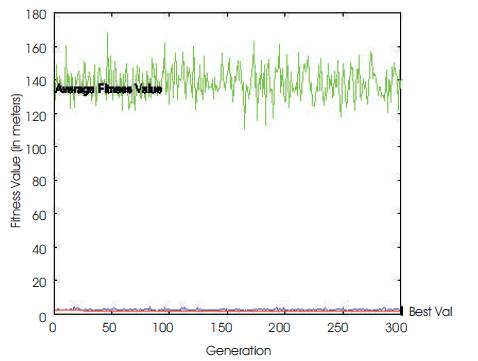
Figure 4. Fitness Value (Best cost results) Vs Population Generation
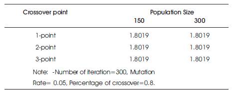
Table 6. Total cost of network in Dollars
In Table 6, the fitness values are very close at one point, two point and three point crossover. Hence single crossover point has been taken.
However, Population size (300), percentage of crossover (80%), number of iteration (300), mutation rate (0.05) and single point crossover parameters have been taken for finding the optimum value (minimum value of head loss) of network. The best nine solutions are given in Table7.
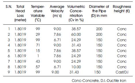
Table 7. Best 9 solutions (Total cost of network in Dollars) that Satisfy Pressure and Demand Constraints
The GA is proposed here for optimal design of slurry pipe network. Simple three-operators of genetic algorithm namely reproduction, crossover, and mutation have been used. Results show that the genetic algorithm techniques are very effective in finding near-optimal or optimal solutions for case study of pipe network. The significant advantages of GA technique are that a set of solutions are produced for decision maker who can choose the optimal alternative solution. The genetic algorithms technique is still in research stage and further development can improve the search method for practical problem.