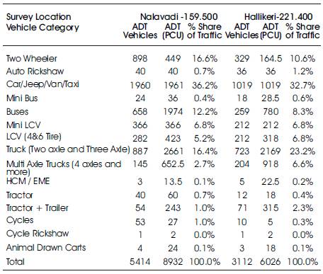
Table 1. Showing Average Daily Traffic
With the recent thrust on improving and developing highways for boosting National Economy, the importance of Traffic Demand Forecasting (TDF) has increased significantly as the forecasted traffic volume contributes substantially in engineering design, economic and financial viabilities of highway improvement projects. Therefore, estimation of traffic growth rates and its related issues concerned primarily to improve the rationality of traffic forecast is of prime importance. In the present Paper, the complete process of Traffic Growth Estimation (TGE)by Transport Demand Elasticity Method even when available data is inaccurate or even missing, merits and demerits of various methods of obtaining traffic growth factors and critical issues associated in the process have been addressed and demonstrated through a case study. It has been revealed that with the constraints of availability of proper data and fluctuation of developing economy, the task of Traffic Growth Estimation could be quite subjective and approximate. Different approaches and necessary considerations for improving the rationality of traffic growth rate have also been addressed in the paper.
The objective of this study is to estimate traffic growth using transport demand elasticity method and to compare how different these values are from the vehicle registration data.
In this present study, an attempt has been made to analyze the O-D data for passenger vehicles (cars & buses) and goods vehicle (trucks) collected by roadside interview method. The passenger characteristics such as average trip length, frequency and freight characteristics are analyzed and tabulated. The influence factors of various zones were found out. Socio-economic data viz -Per capita income and Net State Domestic Product, demographic data such as Population and registration of vehicle data of different states influencing the study stretch were collected from statistical data sources. The relationship between annual growths of vehicles in percentage over number of years is established.
To determine elasticity values, the regression analysis is carried out between socio economic variables growth index and vehicle growth index. The elasticity values for the future years are calculated based on the growth trend of vehicles.
The Project stretch is a part of NH-63 in the state of Karnataka which runs from east to west connecting Karnataka to Andhra Pradesh. The total length of NH-63 is about 432 km, out of which 370 km runs in Karnataka State and about 55.4 km runs in Andhra Pradesh.
This case study deals with Hubli – Hospet stretch of NH-63. The project stretch, starts at km 132+000 of NH-63 at junction with NH-4 Hubli-Dharwad bypass and ends at km 268+700 at junction of NH-63 and NH-13, Hitnal Junction.
For the purpose of forecasting traffic on the study stretch, several primary and secondary data were collected as mentioned below.
On the basis of reconnaissance survey and as per the recommendations of IRC, the project stretch was divided into two homogenous sections and suitable location for each section was strategically selected. The various traffic surveys carried out were:
Strict adherence to IRC codes and manuals were followed for the traffic surveys carried out.
Table 1. Showing Average Daily Traffic
Traffic levels along a study stretch vary during different periods of time i.e., in different months/seasons. Information on this aspect is necessary to estimate the AADT (Table 3). This is best understood by studying monthly historical traffic volumes on the project corridor. This however is not available for the study stretch. In the absence of this direct information, it is customary to consider the monthly sales of petrol and diesel, at the fuel stations along the project corridor or on the road stretches in its environment. This information is presented in Table 2. The factors for passenger vehicles are based on petrol sales and that of goods vehicles (Trucks/LCV's) and buses on diesel sales.
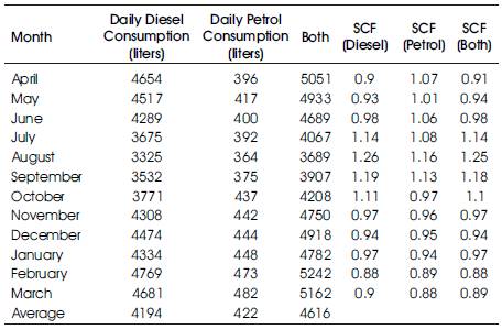
Table 2. Showing daily fuel sales and Seasonal Correction Factors (SCF) required estimating AADT
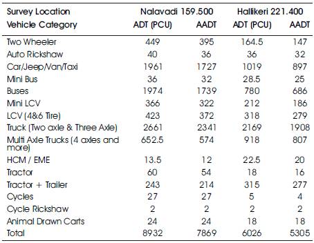
Table 3. Showing AADT obtained after applying Seasonal Correction Factors
To establish the future traffic growth rates, following approaches have been explored.
Past traffic data as collected from PWD is available for two locations (near Annigere and Gadag) along the project corridor. These data are available from January to July months of last 10 years. The growth rates were worked out for various categories of vehicles and conclusions were drawn.
Non-Uniformity in past traffic data of PWD may be attributed to errors during collection and processing of data and policy measures of the Government and other influences etc. To illustrate this point during recent years some of the mining activities around the project corridor have been banned by the Government which has caused a substantial decrease in the amount of trucks and Lorries. As the past traffic data on the Project Road is not showing any definite trend, one should not be guided by past traffic data for deriving growth rates.
An alternative approach is to explore the registered motor vehicles growth in the influence area and assume a growth rate equal to the average growth of vehicle registration. Such an assumption may not be correct, unless the area of influence is well defined and the general development pattern of influence area remains same. The growth rates for various modes are estimated and presented in Table 4. It can be observed from Table 4, during the last 7 years, average growth of two wheelers, cars and that of trucks is around 11%-12%. This high growth rate of more than 10% may not sustain in future. Therefore other rational approaches were explored in order to derive realistic growth rates.
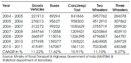
Table 4. Summary of Cumulative Average Annual Growth Rate of Vehicles (%) in Karnataka state7
The exercise of traffic growth rate estimation has been carried out by us using the elasticity approach. The elasticity method relates traffic growth to changes in the related economic parameters. According to IRC-108-1996, elasticity based econometric model for highway projects could be derived in the following form:
Log e (P) = A0 + A1 Log e (EI)
Where:
The main steps followed are:
The results obtained from the Origin Destination surveys were used to identify the project influence area. The ratio of the total traffic originated/destined to a particular zone to the total traffic gives the influence factor for the particular zone. The influence factors were developed from the OD matrices and influence of each State is given in Table 5. A comparative study of the influence factors indicated that Karnataka State, where the project stretch runs has the majority influence of ninety two percent (92%). State of Goa, Andhra Pradesh and Maharashtra that has its border abutting Karnataka State has an influence factor of two percent (2%) four percent (4%) and two percent (2%) respectively. Tamil Nadu/Kerala and Rest of India has minimal or no share at all. These factors have all been accounted in derivation of the combined growth factor and utilized for the project sections.
Elasticity value is the factor by which the socio-economic growth rate is multiplied to get the growth rate of traffic. Traffic is directly linked to the economic growth such as per-capita income, population and NSDP/GDP. Considering the time series data on category wise registered vehicles and the economic variables, by regression analysis elasticity values is estimated as shown in Table 6.
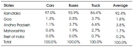
Table 5. Influence of Vehicles observed on the Project Road
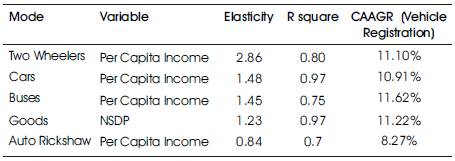
Table 6. Elasticity Values derived based on Regression Analysis for Karnataka State
Based on the moderated elasticity values and the projected economic/demographic indicators and with the given model as follows, the future average annual compound traffic growth rates by vehicle type are estimated.
Passenger Vehicles
Traffic Growth Rate = [ (1+rp) ( 1+ rpci x Em) – 1]
Where,
rp= Population Growth, rpci= Per capita Income Growth, Em= Elasticity
Goods Vehicles
Growth Rate for Goods Vehicles = Elasticity Value * NSDP Growth Rate
The growth rate estimated from elasticity values are shown in the Table 8 below:
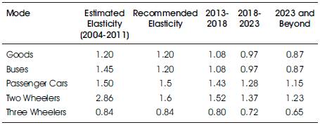
Table 7. Showing adopted Elasticity values for future years
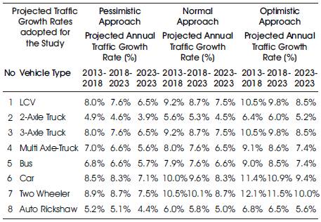
Table 8. Showing Growth Rates adopted for different classes of Vehicles
The comparison of growth rates on vehicular registration data and by elasticity value are as shown in Table below:
The growth rates obtained from transport demand elasticity method is a widely used method all over India. These growth rates are adopted to predict future traffic volumes and Laning requirements.
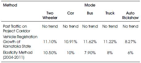
Table 9. Comparison of Growth Rates by Various Methods