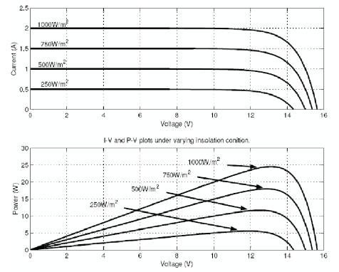
Figure 1. Changes in the Characteristics of the Solar PV Module due to Change in Insolation Level
This study presents a new kind of Maximum Power Point Tracking algorithm based on perturb and observe algorithm. A generalized photovoltaic array simulation model in Matlab/Simulink environment is developed and presented in this paper. The model includes PV module and array for easy use on simulation platform. The proposed model is designed with a user-friendly icon and a dialog box like simulink block libraries. Considering the effect of solar irradiance and temperature changes, the output current and voltage of PV modules are simulated and optimized using this model. A perturb and observe algorithm based maximum power point tracker is also developed using the presented model in Matlab/Simulink. It can successfully track the maximum power point more accurately and quicker than other conventional method based controller in these situations. The general model was implemented on Matlab scrip file, and accepts irradiance and temperature as variable parameters and outputs the I-V characteristic. A particular typical 800W solar panel was used for model evaluation and results.
The photovoltaic modules are made up of silicon cells. The silicon solar cells give an output voltage of around 0.7V under open circuit condition. When many such cells are connected in series, we get a solar PV module. Normally in a module, there are 36 cells which amount for a open circuit voltage of about 20V. The current rating of the modules depend on the area of the individual cells. Higher the cell area, high is the current output of the cell. For obtaining higher power output, the solar PV modules are connected in series and parallel combinations forming solar PV arrays. A typical characteristic curve is called current (I)-voltage (V) curve and power (P) voltage (V) curve of the module [2].
Power output of a Solar PV module changes with change in direction of sun, changes in solar insolation level and with varying temperature as shown in Figures 1 and 2. As seen in the PV (power Vs. voltage) curve of the module, there is a single maxima of power. That is there exists a peak power corresponding to a particular voltage and current. The efficiency of the solar PV module is low about 13%. Since the module efficiency is low, it is desirable to operate the module at the peak power point so that the maximum power can be delivered to the load under varying temperature and insolation conditions. Hence maximization of power improves the utilization of the solar PV module [3]-[5].
Figure 1. Changes in the Characteristics of the Solar PV Module due to Change in Insolation Level
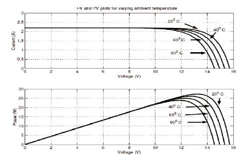
Figure 2. Change in the Module Characteristics due to the Change in Temperature
A Maximum Power Point Tracker (MPPT) is used for extracting the maximum power from the solar PV module and transferring that power to the load. A DC/DC converter (step down/step up) serves the purpose of transferring maximum power from the solar PV module to the load. A DC/DC converter acts as an interface between the load and the module as shown in Figure 3. By changing the duty cycle, the load impedance as seen by the source is varied and matched at the point of the peak power with the source so as to transfer the maximum power [6-7].
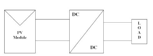
Figure 3. Block Diagram of a Typical MPPT System
As discussed previously, the maximum power point is obtained by introducing a DC/DC converter in between the load and the solar PV module. The duty cycle of the converter is changed till the peak power point is obtained [8]-[9].
Considering a step down converter is used.

where, Vo is output voltage and Vi is input voltage. Solving for the Impedance Transfer Ratio,

where Ro is output impedance and Ri is input impedance as seen by the source.

Thus output resistance Ro remains constant and by changing the duty cycle, the input resistance Ri seen by the source changes. So the resistance corresponding to the peak power point is obtained by changing the duty cycle as shown in Figure 4.
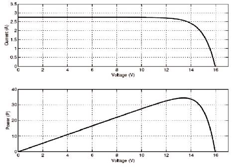
Figure 4. DC/DC Converter helps in Tracking the Peak Power Point
In this algorithm, a slight perturbation is introduced as shown in Figure 5. Due to this perturbation, the power of the module changes. If the power increases due to the perturbation then the perturbation is continued in that direction. After the peak power is reached, the power at the next instant decreases and hence after that the perturbation reverses [10]-[11].
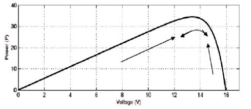
Figure 5. Perturb and Observe
When the steady state is reached, the algorithm oscillates around the peak point. In order to keep the power variation small, the perturbation size is kept very small. The algorithm is developed in such a manner as shown in Figure 6, that it sets a reference voltage of the module corresponding to the peak voltage of the module. A PI controller then acts moving the operating point of the module to that particular voltage level. It is observed that there is some power loss, due to which perturbation also fails to track the power under fast varying atmospheric conditions. But still this algorithm is very popular and simple [12]-[13].
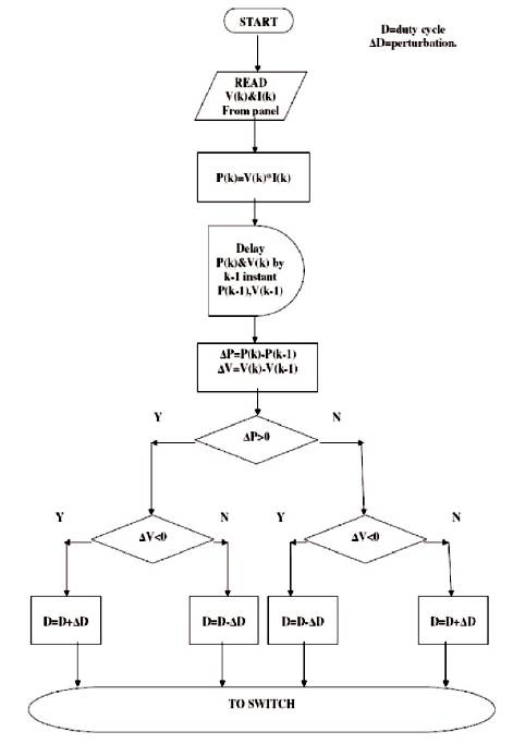
Figure 6. Perturb and Observe Algorithm
There are three basic types of DC-DC converters to track the maximum power from solar PV system to the load. A DC/DC converter is an integral part of any MPPT system. Without DC/DC converter, no MPPT system is designed.
A buck converter is a step-down DC-DC converter as shown in Figure 7. The simplest way to reduce a DC voltage is to use a voltage divider circuit, but voltage dividers waste energy, since they operate by bleeding off excess voltage as heat. A buck converter, on the other hand, can be remarkably efficient (easily up to 95% for integrated circuits) and self-regulating, making it useful for tasks such as converting the 12-24v typical battery voltage down to the several volts needed by the processor [14].
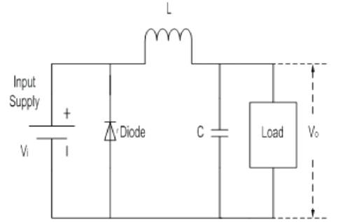
Figure 7. Buck Converter
The operation of the buck converter is fairly simple, with an inductor and two switches (usually a transistor and a diode) that control the inductor as shown in Figure 8. It alternates between connecting the inductor to source voltage to store energy in the inductor and discharging the inductor into the load.
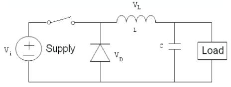
Figure 8. Buck Converter when Switch is Open
A Buck converter operates in a continuous mode if the current through the inductor (I ) never falls to zero during the commutation cycle. The operating principle of this mode is described in Figure 9.
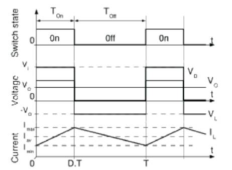
Figure 9. Buck Converter Waveforms
When the switch is closed (On-state), the voltage across the inductor is VL = Vi − Vo. The current through the inductor rises linearly. As the diode is reverse-biased by the voltage source V, no current flows through it.
When the switch is opened (off state), the diode is forward biased. The voltage across the inductor is VL = − Vo. The current IL decreases.
The energy stored in inductor L is,
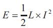
Therefore, it can be seen that the energy stored in L increases during On-time (as IL increases) and then decrease during the Off-state. L is used to transfer energy from the input to the output of the converter.
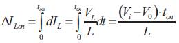
The rate of change of the IL is given by,

With VL equal to Vi − Vo during the On-state and to − Vo during the Off-state. Therefore, the increase in current during the On-state is given by,
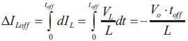
Identically, the decrease in current during the Off-state is given by,
If it is assumed that the converter operates in steady state, the energy stored in each component at the end of a commutation cycle T is equal to that at the beginning of the cycle. That means, the current IL is the same at t=0 and at t=T. Therefore,
So it can be write from the above equations,
As ton = D.T and toff = T – D.T. D is scalar called the duty cycle with a value between 0 and 1. This yields,
The equation above can be rewritten as,

From this equation, it can be seen that the output voltage of the converter varies linearly with the duty cycle for a given input voltage. As the duty cycle D is equal to the ratio between ton and the period T, it cannot be more than 1. Therefore Vo ≤ Vi [15]-[18], [1].
The simulation of solar PV module characteristics is done on the MATLAB/Simulink.
IV and PV characteristics of Solar PV model are shown in Figures 14 and 15.
Open circuit voltage (Voc) = 22.22V
Short circuit current (Isc) = 5.45 A
Current at Pmax = 4.95 A
Voltage at Pmax=17.2 V
Diode “ideality factor” m=2
Thermal Voltage = vT = (k.T/e)
Constant of Boltzmann k= 1.380658*10-23 Jk-1
Charge of an electron e=1.6021733*10-19 as
Insolation= 800W/M2
Figure 10 shows the Matlab model of the PV module and the PV module subsystem has been described in Figure 11.
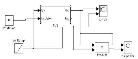
Figure 10. PV Module
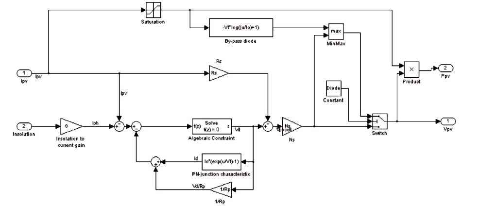
Figure 11. PV Module Subsystem
The MATLAB code computes model parameters Io, Rs , Rp based on the model parameters (short-circuit current Isc, circuit voltage Voc, rated voltage Vr , and rated current Ir). The masked subsystem model parameters are defined as in Figure 12. The initialization step is described in Figure 13.

Figure 12. Subsystem Model Parameters
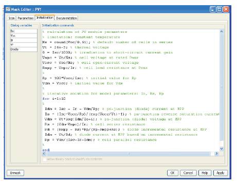
Figure 13. Model Mask: Initialization
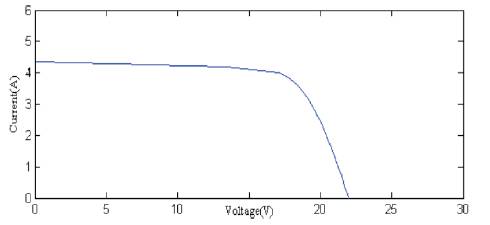
Figure 14. I-V Characteristics of PV Module
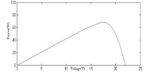
Figure 15. P-V Characteristics of PV Module
PV module at different insolation and their subsystem are shown in Figures 16 and 17 respectively. The characteristics of solar PV Module at Different insolation are shown in Figures 18 and 19.
Insolation = 200, 400, 600, 800, 1000 W/M .
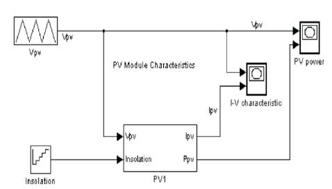
Figure 16. PV Module at Different Insolation
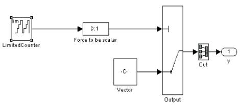
Figure 17. Insolation Mask Sub System

Figure 18. I-V Characteristics of PV Module at Different Insolation
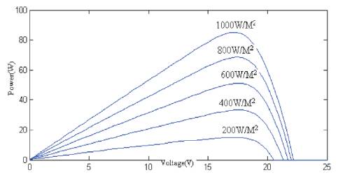
Figure 19. P-V Characteristics of PV Module at Different Insolation
When the module is connected in series, current is same and the voltage is multiplied by the number of solar photovoltaic module connected in series (Figure 20). The I-V & P-V characteristics are shown in Figures 21 and 22 respectively.
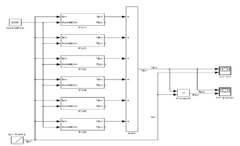
Figure 20. Six Module Connected in Series
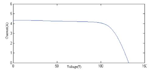
Figure 21. I-V Characteristics of PV Array
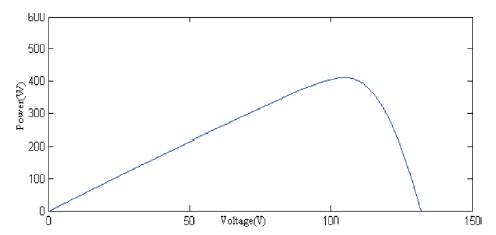
Figure 22. P-V Characteristics of PV Array
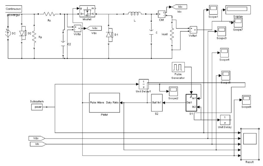
Figure 23. Complete Simulink Model of Perturb& Observe Algorithm
The simulink setup of the MPPT system is shown in Figure 23. The MPPT block takes the module voltage and current through the millimeter. The MPPT block contains the algorithm which is explained below in Figure 24. The insolation and the temperature are kept fixed and are not varied. For implementing the perturb & observe (P&O) algorithm, the value of all the components are given as,
PV Pannel specification
Light generated current Iph =5.6 A
PV Series resistance Rs=.1 ohm
PV Parallel resistance Rp=64.413
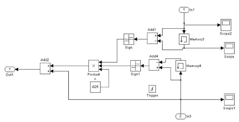
Figure 24. Algorithm Implementation in Simulink (S1) for Duty Ratio
L=.01 H
C=.00050 F
Figure 25 shows the power vs time. Initially power drawn from solar panel is less. Then duty ratio is increased via algorithm. Figure 26 shows the voltage versus time. Initial condition is more towards open circuit condition due to which the voltage is high. As duty ratio increases, current drawn (Figure 27) from solar panel increases which result in drop in voltage.
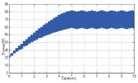
Figure 25. Power Vs Time
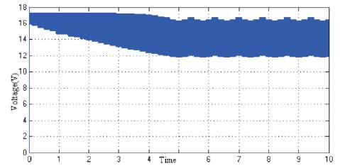
Figure 26. Voltage Vs Time
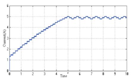
Figure 27. Current Vs Time
Finally, when the power is reached to the maximum point, duty ratio is set (Figure 28) and the power is oscillated around the maximum power. Here maximum power is 82 watt.
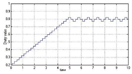
Figure 28. Duty Ratio Vs Time
Figure 29 shows the pulses which are generated by the perturb and observe algorithm of maximum peak power point, and these pulses are used to drive the switch (MOSFET) of the DC Buck converter for extracting the maximum power from a solar photovoltaic module.
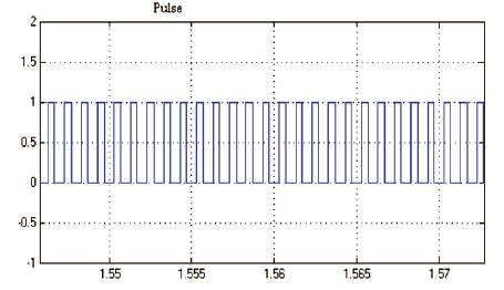
Figure 29. Switching Pulse for the Switch of the Buck Chopper
P&O MPPT method is implemented with MATLAB-SIMULINK for simulation. The MPPT method simulated in this paper is improves the performance of the PV system simultaneously. Through simulation, it is observed that the PV system completes the maximum power point tracking successfully despite of fluctuations. When the external environment changes suddenly, the system can track the maximum power point quickly. Buck converter is much more effective specially in suppressing the oscillations produced due the use of P & O technique.
With an increase in demand for electric energy, there is a need to search for an alternative source of power generation as the conventional sources of energy have started to get depleted. The solution for this problem is the concept of renewable energy source. Solar, tidal, wind, etc. comes under renewable energy sources. In the 21stcentury, electric power generation undergoes dramatic changes in both physical infrastructure, and control information infrastructure. Power electronics technology plays an important role in distributed energy generation. The advent of high power electronic modules has encouraged the use of more DC transmission and made the prospects of interfacing DC power sources such as photovoltaic and fuel cells. A change will take place from a relatively few large, conventional generation centers and transmission of electricity to more diverse and dispersed generation and transmission. A new kind of maximum power point tracking algorithm based on perturb and observe algorithm an be used. The algorithm is fast acting and eliminates the need of a large capacitor which is normally used to eliminate the ripples in the module voltage. The module voltage and current that are taken for processing are not averaged but are instantaneous which speed ups the process of peak power tracking. Analyzing and designing DC/DC converters of different types in a solar energy system is carried out to investigate the performance of the converters. This simple method which combines a discrete time control and a PI compensator is used to track the Maximum power points (MPP's) of the solar array. The system is kept to operate close to the MPPT's, thus the maximum possible power transfer from the solar array is achieved
A complete generalized model of PV array along with perturb and observe algorithm based MPPT controller has been developed in Matlab/Simulink in this paper. The specialty of this perturb and observe algorithm is that it is very simple. That is why the proposed perturb and observe algorithm can track the MPPT very fast and accurately even if the environment changes abruptly. The performance of the proposed controller is better with other conventional controller. The proposed controller can be used in any real PV system. This controller gives a better output value for buck. Hence this controller will give different kind of curves for the entire converter. In simulation, Buck converter shows the best performance, and the controller works at the best condition using a buck converter. The algorithm is fast acting and eliminates the need of a large capacitor which is normally used in perturb and observe algorithm to eliminate the ripples in the module voltage. The module voltage and current that are taken for processing are not averaged but are instantaneous, this speed up the process of peak power tracking. Also the paper implements the new algorithm on the real time platform.