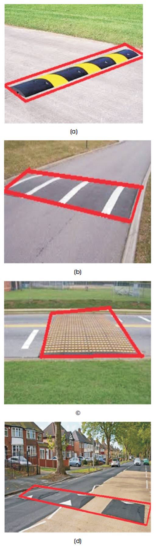
Figure 1. Types of Speed Breakers, (a) Speed Bumps, (b) Speed Humps, (c) Speed Cushions, (d) Speed Tables
Road bumps are elevated pavements placed transversely to the road, forcing the driver to reduce the speed of their vehicles. They play a crucial role in increasing safety at sharp curves, residential streets and accident prone areas by controlling the speed of the vehicles. The amount of speed reduced mainly depends on length, height, and type of speed breakers. Major types of speed breakers generally adopted are speed bumps, speed humps, and artificial speed breakers. This paper aims to find the variation of speeds of different class of vehicles at speed breakers and to develop a model for finding the bump height that should be provided at that particular road for a given safe speed limits of different types of vehicles on that road section. To achieve this, three locations were selected, two locations in Hyderabad and one location near Autonagar area of Vijayawada city. Volume counts for the above roads were observed for every 15 -minute intervals. The video was recorded during peak hours and the variation of speeds before and after 10 m from speed breakers were calculated at these locations. The average reduction in speed of vehicles with respect to the approaching speed at the distance of 10 m from bump is 52.69% at KPHB, 64.5% at ORR, and 39.26% at Vijayawada.
Traffic safety is an important aspect in the design and maintenance of roads. But with an increase of the world population traveling by road, a more vigorous understanding of road traffic safety becomes necessary. Speed is the fundamental measure of traffic performance of a roadway system as it indicates the excellence of service experienced by the traffic stream. Speed bumps, also known as road bumps, are widely utilized for controlling vehicular speed and enhancing the traffic safety at accident prone areas. Unnecessary provision of speed breakers lead to irritation and discomfort of road users (Philip and John, 2005). According to the Road Accident Report (2015), published by the Times of India, every year 4,726 lives were lost in crashes due to road humps while 6,672 people died in accidents caused due to potholes and speed breakers. Speed breakers should be only provided, where more accidents are happening due to over speeding. The amount of speed reduction depends on various types of speed breakers. They are listed below and shown in Figure 1.
Figure 1. Types of Speed Breakers, (a) Speed Bumps, (b) Speed Humps, (c) Speed Cushions, (d) Speed Tables
The literature review on speed breakers involves a wide range of investigations on the development of speed bump systems. Speed bumps are of different types, a similar study was conducted on speed humps, speed slots, and speed cushions by Latoya and Nedzesky (2004), the driver behavior across speed cushions and bumps were analyzed and speed analysis has been conducted. It was observed that the speed humps allow a highest average of 85th percentile speed than speed bumps. Ponnaluri and Groce (2005) studied the speed variations before and after installation of speed breakers. A model was developed by Sahoo (2009) for anticipating bump crossing speed based on area to width ratio. David (2012) gave a brief idea about how width of speed bump can influence the speed reduction of vehicle. He concluded that, for effective functioning of speed bumps, the ratio of width of the road to the width of bump should be less than one for an operating speed range of 25-30 km/hr. This study also concluded that the use of small bump width is more appropriate than wider bump width. Zainuddin, et al. (2012) conducted a study about optimization of speed bump with length, width, and height. Ashish (2013) gave a brief idea about the speed bumps and he used radar gun to estimate the speed of the vehicles by the radar signals caused by Doppler Effect. Parvathi, et al. (2013) have used microsimulation software VISSIM 5.40 and concluded that provision of speed bumps decreases the level of service as travel time is increased due to reduction in vehicular speed. He also noticed that average speed of vehicles for two wheelers and four wheelers is more than that of heavy vehicles. Speed bumps should be located at proper locations otherwise, it causes more traffic problems. Alireza, et al. (2013) conducted a study for finding the best location for placing of speed bumps. To evaluate the design data, software was utilized and it also depends on some restraint factors like car weight, car speed, and surface inclination. He also stated that width of speed bumps will have an effect on operating speed. A homogeneous traffic flow model was developed by Ashutosh Gundaliya (2015) which features the vehicle generation, lane changing criteria, model calibration and validation.
For analyzing the speed profile at speed breakers, three locations were considered. The methodology adopted at these locations can be explained with the help of flowchart shown in Figure 2.
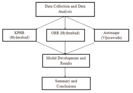
Figure 2. Flowchart of Methodology
Three locations were chosen for analysing the speed profile analysis and the photographs of the site selected are shown in Figure 3.
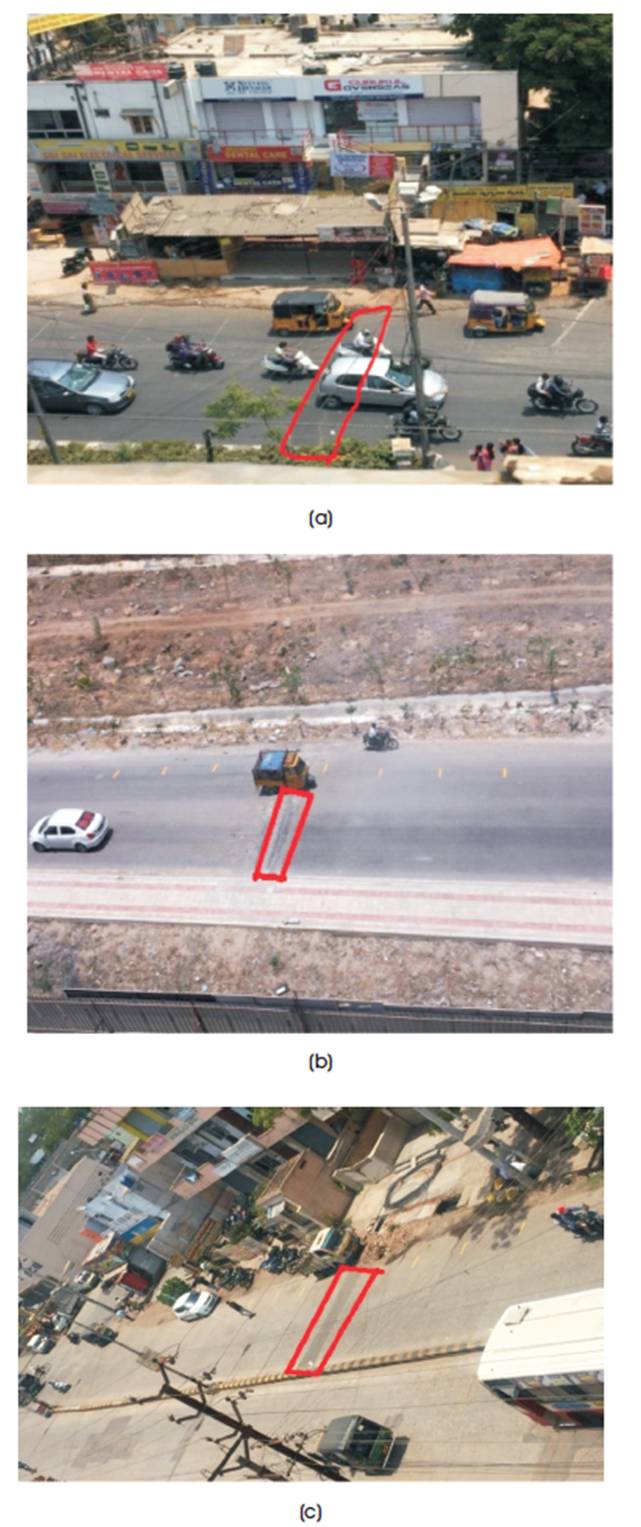
Figure 3. Project Locations, (a) KPHB Location (Hyderabad), (b) Outer Ring Road (Hyderabad), (c) Autonagar (Vijayawada)
At each of the above selected location, road geometrical features were recorded and shown in Table 1.
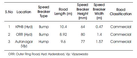
Table 1. Road Geometrics
Video camera technique was used to record the details. Camera was put in an elevation so that, all data can be extracted easily without any disturbances. Video was collected for a three-hour duration during peak hours. Data for vehicles travelling in both ways were collected. At each speed breaker location, 20 m span was chosen such that, 10 m was before speed breaker and 10m was after speed breaker. This 20 m span is divided into 7 intervals. Among the 7 intervals, 6 were of 3 m span and one interval is of 2 m at exact speed bump location. This 2 m span was considered for calculating the vehicular speed at speed bump.
From the videos recorded at each location, volume was directly extracted by counting and speed was extracted indirectly by measuring the travel times of vehicles between each interval and the distance between those intervals. Average vehicular volume was extracted at each location for a duration of 3 hours in peak duration and it is shown in Table 2.
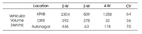
Table 2. Average Vehicular Volumes at each Location
The time taken by each vehicle to travel in the respective intervals were recorded and correspondingly the speed is calculated and is shown in Table 3.
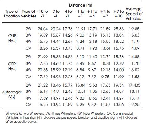
Table 3. Variation of Vehicular Speed at each Interval
Speed was calculated at seven different intervals defined on the bump at 10 m, 7 m, 4 m, and 1 m before and after the speed breaker. Average speed of vehicles at the selected intervals is shown in Figure 4.
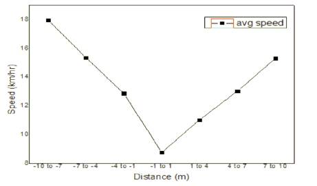
Figure 4. Average Speed Profile of Vehicles at a Speed Bump
Average vehicular speeds at all three locations are compared with bump heights and is shown in Figures 5, 6, 7, and 8 for 2 wheelers, 3 wheelers, 4 wheelers, and commercial vehicles, respectively.
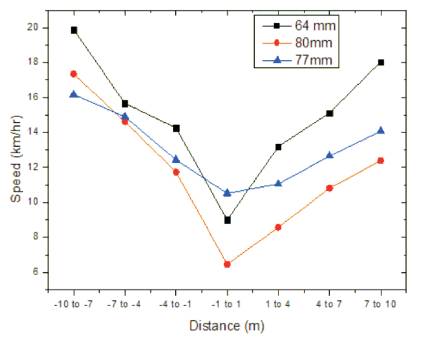
Figure 5. Comparison of 2W with Bump Height
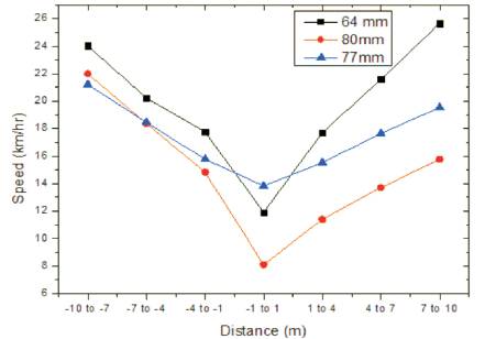
Figure 6. Comparison of 3W with Bump Height
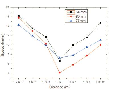
Figure 7. Comparison of 4W with Bump Height
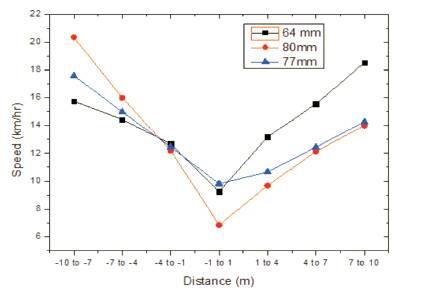
Figure 8. Comparison of CV with Bump Height
Reduction of vehicular speeds for 2 wheelers, 3 wheelers, 4 wheelers and commercial vehicles at each location is calculated and shown in Table 4.
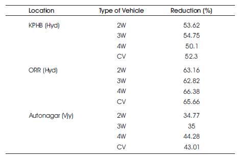
Table 4. Reduction of Speed
It is a statistical hypothesis test. It can be used to govern if two sets of data are considerably dissimilar from each other. The P-value for T test can be attained from Microsoft excel using T test function and it is provided in the Tables 5, 6, 7, and 8.
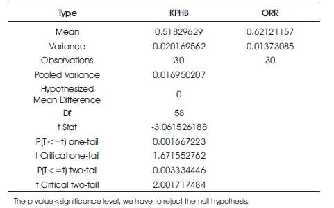
Table 5. T Test for 2 Wheelers in KPHB and ORR Location
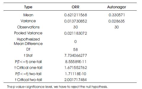
Table 6. T Test for 2 Wheelers in ORR Location and Autonagar location
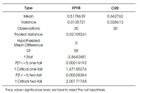
Table 7. T Test for 4 Wheelers in KPHB and ORR Location
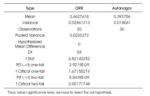
Table 8. T Test for 4 Wheelers in ORR Location and Autonagar location
From the t-test results, the authors tabulated the reduction attained by bump height under diverse locations as in Table 9.
Table 9. T-test Conclusion for different Vehicles
A MLR (Multi Linear Regression) model was developed by taking bump height as dependent variable and average speeds of 2 wheelers, 3 wheelers, 4 wheelers and commercial vehicles as independent variables. To develop the model, all the three locations data was considered and given as an input to SPSS software. The equation developed for fixing the bump height for a given speed values is as follows:
Bump height = 86.791-0.293*W2-0.454*W3-0.468*W4 +0.353*CV
where W2 = Average speed of 2 wheelers,
W3 = Average speed of 3 wheelers,
W4 = Average speed of 4 wheelers,
CV = Average speed of Commercial Vehicles.
The R2 value obtained for the above equation is 0.873.
For validating the above obtained equation, vehicular speeds at the Autonagar location were considered and bump height was calculated from the model developed.
Bump height = 86.791-0.293*W2-0.454*W3-0.468W4+ 0.353*C
= 86.791-0.293*(14.45)-0.454*(13.40)- 0.468*(12.44)+ 0.353*(18.23)
= 77.093mm
The bump height provided at that location was 77 mm and the height obtained from the model was 77.093 mm, which shows the model developed was reasonably good and can be used for calculating the bump height at various locations.
Based on the analysis and results, the following conclusions are drawn: