[1]

The Hydroelectric power is generated by the rotating turbine through high pressure falling water that drives the generator. So far as electricity production is concerned, hydro-power is the most established and popular renewable resource. As a matter of fact, hydro-turbines have a very quick response for power generation and thus they are capable of handling the load variations. Besides, these can be directly connected to the grid. Among the renewable sources, Micro Hydro Power (MHP) is attractive because of its mature technology, spallation cheap cost, minimum civil work, manageable technology which is robust and reliable that it is applied for controller, generator, and turbine technologies. In this paper, a 60 KW, 132 KV synchronous generator with two controllers are designed and simulated to control the mechanical power input and another controller for controlling the excitation of synchronous generator and synchronous generator output at 13.8 KV is fed to load of 2 KW at 13.8 KV and then this 13.8 KV is stepped down to 400 V to feed the loads of 10 KW and 50 KW. Here 10 KW load is connected through the breaker, to provide load variations and 50 KW load of fixed type.
The small size generator (<100 KW), the governor action makes free flow of water which is not incorporated to hit the turbine. Small Hydro Power (SPH) plants and Micro Hydro Power (MHP) plants have acquired increase in attention owing to ecological irresponsibility and responsible prices for the generation of sufficient electric power without production of unexpected obnoxious pollutants, including greenhouse gases [30], [32]. In MHP and SHP plants, the power generation is converted to stable electric power sources by high power semiconductor devices with good power quality in order to meet commercial load requirements by novel AC to DC converters and DC to AC inverters [29], [36]. Micro hydro turbines under 100 KW power topologies of micro hydro generation, fixed speed generation, direct-connected grid integration topology, variable speed generation, and Power electronics grid integration topologies was studied [3].
Micro Hydro Power generation systems facilitate about the carbon dioxide, emission reduction, and supplies energy with diversification. The components of MHP system are generator turbine blades, generator brackets, and control systems [13]. Vertical blades micro hydro power turbine, bearing and a generator are the construction features of a micro hydro power turbine. The maximum power output is achieved by complete submission by setting the water level above turbine blades [11]. Output power is directly proportional to the blades in which squared area is passed by water, therefore if the blades are submerged completely, the maximum turbine output is achieved [6]. In order to improve efficiency of operation and power grid integration from economical and technical point of view,
the power systems like wind, tidal or even micro hydro are needed from large and small power plants, more than 19% of hydroelectric power provides electricity consumption of the world, the word “Micro Hydro” has no universally accepted definition, which depends on local definitions and varies from a few kilo watts up to 100 KW [10], [19].
The electrical configuration includes power interface which depends on chosen generator and power grid. The classical structure control system separates two subsystems which is decoupled by a power electronics interface [17]. The generator side as well as control loop is delayed with the operation of turbine and control loop of grid side, which ensures the transfer of power generated to grid utility Hydraulic turbine is coupled rigidly by PSMG electrical machine of few kilowatts. Power electronics converter consists (VSI) back to back two level voltage source inverter utilised by an interfaced generator [33], [35]. The grid-side converter connects utility via an AC power transformer. The conversion of falling water gravitation energy to mechanical power is done by the turbine [24]. The available (Potential) hydraulic power expression which depends on water head besides flow rate (discharge) can be expressed as,
The mechanical power which is exhaustible is given by,

where PT is mechanical power produced at the turbine shaft (watts),η is efficiency of hydraulic turbine,ρ is volume 3 density of water (kg/m ), g is acceleration due to gravity 2 3 (m/s ), Qw is flow of water (m3/s), H is head of water across the
turbine (metres) [26]. Operational functions of water flow and shaft speed and head determines the efficiency of the hydraulic turbine [18].
The interface between the generator and the unit grid is implemented by PWM power electronics converter and the generating system was divided into two separate plants [1]. The control structure has three levels, i.e., the innermost layer, intermediate layer, and outermost layer. The innermost layer consists of control over both inverters as current control [2]. The intermediate layer based on generator sides converter and DC-bus voltage control with rotational speed control and the outermost control loop have many functions like supervision, optimization operation protection, and auxiliary services eventually. The control strategy in grid-connected mode performs the task by two converters [25]. The DC-Bus voltage at a constant value is maintained by grid side, converter at a constant value to evacuate electricity. Micro hydropower has several advantages compared to solar wind power, i.e. it has long lasting and robust technology [20], [21].
The main objective of the paper is to develop a micro hydro plant with PID controller which can be connected directly to the grid and can withstand variations in load and supplies to load immediately. These micro hydro projects can be constructed in places of mountains and hilly areas where water availability is present and because of its mature technology and construction is also limited. It can be used to supply base load as well as peak load. Power generation can be varied with changes in load demand. It is being tried to implement in different loadings i.e., under load and over load conditions in order that system should be stable and supply accordingly. The controlling technique used is PID governor including pilot and servo dynamics as it is required to increase regulation under fast transient conditions for achieving stable speed control. This can be achieved by parallel transient droop branch with time constant TR and implementing the power quality can be improved by using the controller in which pure sinusoidal waveform is obtained. Harmonic content can also be reduced. The sharing of load will be observed with increase and decrease in load with variations in speed of the turbine. Active power and reactive power at different loadings will be observed and load sharing will be done.
Figure 1 shows the basic elements of hydro turbine within the power system environment. However, models for generation load control and electrical and dynamics are excluded [25].
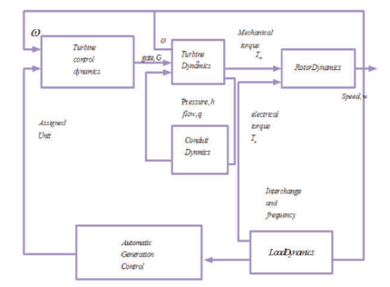
Figure 1. Functional Block Diagram showing Relationship of Hydro Prime Mover System and Controls to Complete System
Figure 2 embodies the dynamic characteristics of a simple hydraulic turbine, with unrestricted head and tail race, a penstock and with either a very large or no surge tank [14].
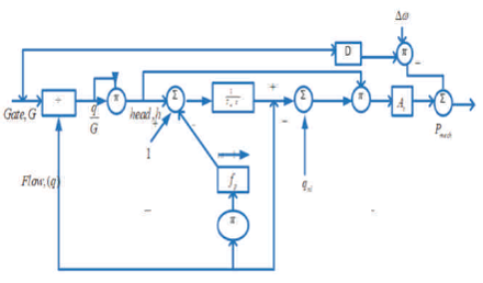
Figure 2. Non-Linear Model of Turbine - Non-Elastic Water Column
The penstock is modelled assuming an incompressible fluid and rigid conduit of length L and cross-section A. Penstock head losses are proportional to flow squared and f is the head loss coefficient, usually ignored [23].
From the laws of momentum, the rate of change of flow in the Conduit is,

where q=turbine flow rate, m /sec, A= Penstock area in m , L= Penstock length in m, g= is the acceleration due to 2 gravity in m/sec , h is the static head of water column in m, 0 h is the head at the turbine admission, m, h is the head loss l due to friction in the conduct m.
Expressed in per unit, this relation becomes,

where h and hi are the head at the turbine and head loss, respectively in per unit, with hbase defined as the static head of the water column above the turbine. Tw is called water time constant or water starting time defined as,

where qbase is chosen as the turbine flow rate with gates fully base open (Gate position G=1) and head at the turbine equal to hbase . It should be noted that the choice of base quantities is base arbitrary [16], [27].
The system of base quantities as already defined is having the following advantages,
Base head (hbase) is simply identified as the whole existing base “static head” (i.e. lake head minus tailrace head).
Base gate can, without doubt, be understood as the maximum gate opening [34].
After discussing about base head and base gate position, the turbine characteristics describe base flow through the relationship,

The per unit flow rate through the turbine is given by,

In an ideal turbine, mechanical power is equal to flow times head with appropriate conversion factors.
The fact that the turbine is not 100% efficient becomes established by subtracting the no load flow from the actual flow giving the difference as the effective flow which, when multiplied by head, does produce mechanical power, damping effect which is a function of gate opening [24].
There is also a speed deviation per unit turbine power P , on m generator MVA base is thus,

where qnl is the per unit no-load flow, accounting for turbine nl fixed power losses. At is a generator MVA base.

where hr is the per unit head at the turbine at rated flow and r q is the per unit flow at rated load.
It should be noted that the per unit gate would generally be less than unity at rated load. Nevertheless, in some stability programs, A is used to convert the actual gate position to t the effective gate position, i.e. At =1/(GFL –GNL ). A separate factor is then used to convert the “p”, from the turbine rated power base to that of the generator volt-ampere base, where GFL is the gate opening at full load and GNL is the gate opening at no load [8].
From Figure 3, the change in mechanical power output can be expressed as,

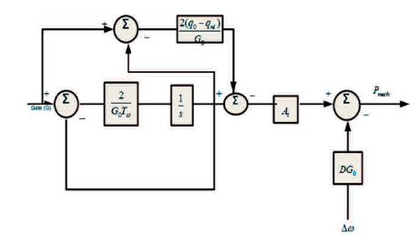
Figure 3. Linearized Model of Turbine - Non-Elastic Water Column
where
G = per unit gate opening at operating point
T1 =(q0 -qnl ) TW
T2=(G0TW/2)
q0 = per unit steady state flow rate at operating point
Note that G0 =q0 .
With the damping term neglected, equation (9) is similar to the commonly used classical penstock/turbine linear transfer function.

where G0TW is an approximation to the effective water 0 W starting time for small perturbations around the operating point. The dynamics of turbine power are an almost instantaneous function of head across the turbine and gate or nozzle opening including deflector effects were applicable [15]. The head across the turbine is a function of the hydraulic characteristics upstream of the turbine and also downstream in cases where the flow in the draft tube and/or tailrace is constrained as in the case of Francis or Kaplan Turbines [12]. In the case of Pelton (impulse) turbines, the downstream pressure is atmospheric, hence the hydraulic effects are only from the conduits between the reservoir and turbine [9].
Particular hydraulic conduit arrangements may require special modelling in cases such as constrained or vented tunnels. Individual penstocks fan out from a common pressure shaft [7]. In this context, the basic models for conduits can be assorted in order to describe the precise arrangement, even as the basic models of electric components are employed to depict specific networks [27].
For their initial inverse response characteristics of power to gate changes, the hydro turbines require stipulation of transient droop features in the speed controls for a stable control performance. By 'transient droop' it is understood that for fast deviations in frequency, it is the governor which exhibits high regulation (low gain) whereas for slow changes, that also in the steady state, the governor of course exhibits the normal low regulation (i.e., high gain) [22], [28]. From the point of view of linear control analysis, a pictorial description of a hydro turbine generator providing an isolated load is shown in Figure 4.
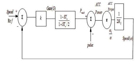
Figure 4. Linear Model of Hydro Turbine and Speed Controls
The model of the typical hydro turbine generator is shown in Figure 5 and the physical meaning of the parameters used in the model is as follows,
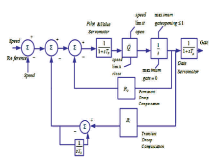
Figure 5. Model of Typical Hydro-Turbine Governor
TP - Pilot valve and servo motor time constant
Q - Servo gain
Tg - Main servo time constant
RP - Permanent droop
RT - Transient droop
TR - Reset time or dashpot time constant.
Due to the peculiar dynamic characteristics of the hydraulic turbine, it is necessary to increase the regulation under fast transient conditions in order to achieve stable speed control. This is achieved by the parallel transient droop branch with washout time constant TR . In vision of the choice of the per unit system, with maximum gate opening defined as unity, the speed limits must be defined, for consistency, as fractions of the maximum gate opening per second [4]. The inverse of the feedback path is 1/hi.

and the forward function g is given as,

The Closed Loop Response (C.L.R.),

If g1 <<1/h1 then: g1h1 <<1 and C.L.R. is approximately = g1
If 1/h1<
Hence, the closed loop response may be approximated by plotting both g and 1/h1 and choosing the lowest of 1 1 both gain responses at any frequency as an approximation to the closed loop response at that frequency, the speed regulating control loop will "see' the governor as having a gain of 1/RP in the steady state, and a 'transient' gain of I/RP for phenomena above the 1/TR frequency range. An R equivalent time constant of 1/(QRt) seconds will result from t the second intersection of the g and 1/h traces.
The speed regulating loop will have acceptable stability, if:
The transient gain (1/Rt) does not exceed,

Crossover frequency, Wc, approximately equal to 1/(2HRt) occurs somewhere in the region between 1/TR and QRt . It reduces phase lag contributions from the governor.

Rise time, TR

For crossover frequencies in the order of 1/2TW , 1/TR values in the order of 1/5TW will minimize ‘low frequency’ phase lag contributions from the governor.
The differences may be due to added time constants in hardware and also where derivative action is included. Figure 6 shows an example of more complex representations.
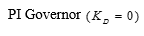
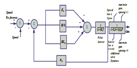
Figure 6. PID Governor including Pilot and Servo Dynamics
Neglecting the pilot servo and additional servo dynamics in Figure 6, the inverse of the internal loop feedback path 1/h1 i.e. 1/Rp and the forward gain g, i.e. KP +Kt/s. Transient droop R is given by 1/kp . Kp/Kl is equivalent to the dashpot time constant TR and care must be taken that crossover R does not occur at frequencies that are close to the inverse of the smaller servomotor time constants [22].
The purpose of the derivative is to extend the crossover frequency beyond the constraints imposed on PI governors. The governor loop frequency response when the PID governor is tuned according to (16).


Transient gain (1/R ) has been increased by 60% over t normal PI values. This results in roughly the same increase in crossover frequency, and thereby, in governor response speed [31].
As it is clear, detrimental effects on stability are averted by the phase lead effects resulting from derivative action. There is a risk, however, that the rise in magnitude due to the derivative action, compounded with that resulting from the hydraulic system may result in a second crossover.
At higher frequencies due to the high phase lags at these frequencies, a second crossover will certainly result in governor loop instability. This is the reason for the minimum limit imposed on the value of KP/KD.
Power conditioning diagram of micro hydro based power generation system is shown in Figure 7. In this system, two controllers are designed to control the mechanical power input and another controller for controlling the excitation of synchronous generator and synchronous generator output at 13.8 KV is fed to load of 2 KW at 13.8 KV and then this 13.8 KV is stepped down to 400 V to feed the loads of10 KW and 50 KW. Here 10 KW load is connected through the breaker, to provide load variations and 50 KW load of fixed type. Figure 8 shows the control circuit diagram of micro hydro system.

Figure 7. Circuit Diagram of Micro Hydro system
Figure 8. Control Circuit Diagram of Micro Hydro System
In Figure 9, time (s) lies on x-axis and input power on y-axis. Here at 90% of loading, the power is maintained at 54 KW and at 108% loading, the power is maintained at 64.8 KW. So the designed system can withstand 90% load and also overload 108% load.
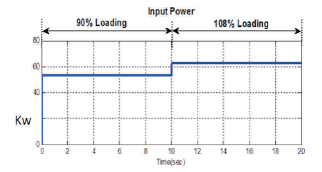
Figure 9. Input Power
From Figure 10, it is observed that the turbine rotational speed increases in 90% loading and in 108% loading, the turbine rotational speed decreases. Whereas the turbine output power and gain position is decreased during 90% loading and increased during the overloading.
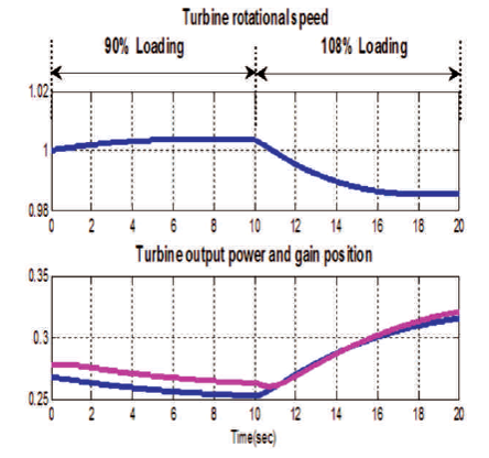
Figure 10. Turbine Rotational Speed and Turbine Output Power
From Figure 11, the voltage is maintained constant both in 90% loading and 108% loading condition is 11.2 KV and the current is maintained constant both in 90% loading and 108% loading condition is 0.1A.
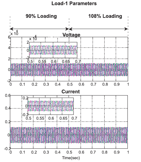
Figure 11. Load 1 Parameters
Figure 11 shows the maintaining of a maximum value of phase voltage as 11.2 KV, (11.2*1.732)/1.414=13.8 KV (rms line value). Figure 12 shows that the real power is maintained constant as 4.8 KW and reactive power is maintained zero both in 90% loading and 108% loading condition.
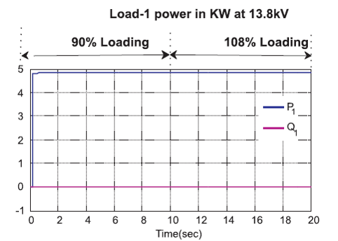
Figure 12. Load-1 Power at 13.8 kV
Figure 13 represents the active power 50 KW to 60 KW is increased from 90% loading to 108% loading condition, whereas reactive power is maintained zero in both 90% and 108% loading conditions as mentioned in the x-axis and y-axis.
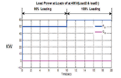
Figure 13. Load Power at Loads of at 400 V (Load 2 & Load 3)
From Figure 14, Real powers are maintained at 50 KW both in 90% loading and 108% loading conditions and the reactive power is maintained constant at zero.
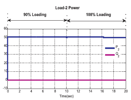
Figure 14. Load-2 Power in Micro Hydro System under Load Varying Condition
From Figure 15, it is observed that the voltage is 326 V maintained constant both in 90% loading and 108% loading conditions and current 100 A is maintained constant both in 90% loading and 108% loading conditions. The max value is 326 volts, (phase value) so maximum value= (326*1.732)/1.414=400 V (rms line voltage).
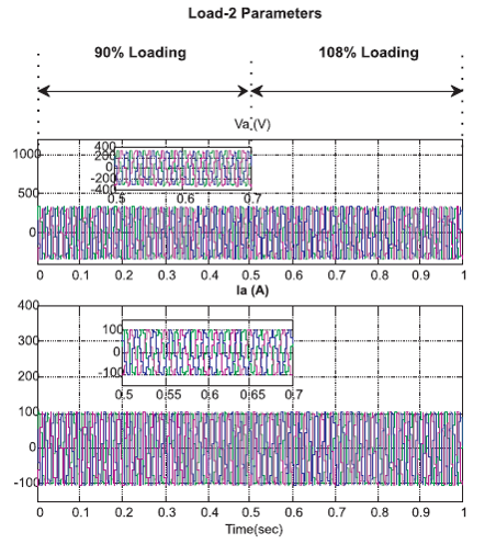
Figure 15. Load 2 Parameters in Micro Hydro System under Load Varying Condition
In Figure 16, after 10 load-3 is on to the system10 kW so 108% loading is maintaining a real power shown in kW from 10 to 20 s and reactive power is zero, which is maintained constant both in 90% loading and 108% loading conditions.
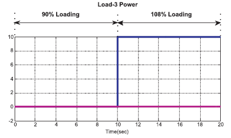
Figure 16. Load-3 power in Micro Hydro System under Load Varying Condition
From Figure 17, no voltage at 90% loading, after 10 s, load 3 is on to the system10 KW and voltage exists at 108% loading and no current in 90% loading condition and 20 A. It is observed that up to 10 seconds, there is no load on the system. Since there is no voltage and current but the load in on from 10 seconds so the two parameters of voltage 326 V and current of 19 Amps were obtained.
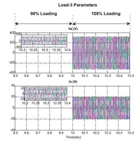
Figure 17. Load-3 Parameters in Micro Hydro System under Load Varying Condition
In Figure 18, it is shown that the voltage is maintained 326 V both in 90% loading and 108% loading and current is raised from 90% loading to 108% loading conditions.
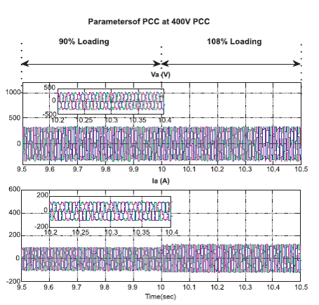
Figure 18. Parameters of PCC at 400 V PCC in Micro Hydro System under Load Varying Condition
This paper discussed the functioning of the power conditioning system for Micro-hydro power generation developed by the researcher for the purpose of study along with the use of some existing systems. In this excitation controller and governor controller are used so that it would fulfill the designed parameters. It has been found that the turbine rotational speed increases in 90% loading and the turbine rotational speed decreases in 108% loading. However, the turbine output power and gain position decreased during 90% loading and increased during the overloading. The parameters of PCC at 400 V PCC was graphically represented to show the real as well as the projected output under simulated conditions. It was further observed that the voltage is maintained 326 V both in 90% loading and 108% loading conditions and current is raised from 90% loading to 108% loading reactive power is zero maintained constant both in 90% loading and 108% loading.
This methodology can be implemented in mountain terrain or hilly areas, which is very useful for power generation where water is available and power can be used for local areas and it can also act as a micro grid. It has advantages of adding it directly to the grid and it can withstand fast variations in the load. The controller used is PID controller including pilot and servo dynamics. The latest controllers fuzzy logic, neural networks, adaptive controllers, ANN, FPGA, etc., can be implemented. Similarly in many locations, watercourse size will swing seasonally. During summer, there will likely be less flow and less power output hence a hybrid system can be designed by using the existing resources.