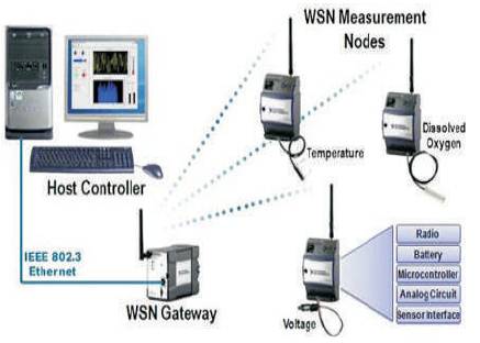
Figure 1. Block Diagram of WSN
In this paper, the authors propose a fully reused high performance architecture to meet the needs of Radio communication which plays a vital role in the Wireless Sensor Nodes. These architectures utilize low power for their operation. In existing architecture the sensor nodes have limited potential to put the tradeoff between processing elements and design. The existing architecture has limited Processing Elements (PEs) that consumes less power and this existing architecture is used for off-the-shell low power microcontrollers which are not preferred for WSN. Most of the Wireless Sensor Network applications require the data to be processed at on-the-node processing. On-the-node processors consumes more power which is major limitation in VLSI. To overcome this limitation and extend the applications of their work, they have used suitable processing elements by taking the advantage of Folded-tree architecture which uses Parallel-prefix operations and thus power consumption is greatly minimized. The design is developed by using the Advanced Simulation and Synthesis tool Xilinx14.3 Design suite and Virtex6 FPGA for hardware Prototyping Environment. The design summary and synthesis report show that the proposed architecture consumes low power and works with high performance.
Wireless Sensor Network (WSN) [9] applications vary from medical monitoring to Environmental sensing, industrial scrutiny, and military police works. WSN nodes primarily contains sensors, a radio, and a microcontroller combined with a restricted power offer e.g., battery or energy scavenging. The goal of this paper is to style associate ultra low-energy WSN digital signal processor by exploiting this and different characteristics distinctive to WSNs.
A Wireless Sensor Network (WSN) may be a wireless network consisting of spatially spread and dedicated autonomous devices that use sensors to watch physical or environmental conditions. A usual WSN system is made by combining these autonomous devices, or nodes with routers, and an entrance. The spread measure nodes communicate wirelessly to a central entrance, that provides an association to the wired world wherever one will be able to collect, process, analyze, and transfer their measured information. One will also be able to use routers to realize an extra communication link between finished nodes and therefore the entrance for extend distance and responsibleness in an exceedingly Wireless Sensor Network [3].
The wireless sensor is networked and scalable, which needless of low power. It is sensible and code programmable and conjointly capable of quick information acquisition, reliable and correct over the long run, however the prices are very low to install and needs Zero maintenance. Wireless Sensor Network is completely different from previous Network. WSN suggests to serve only specific applications whereas previous network suggests for serving several applications.
Energy is the main constraint within the style of all node and network parts in Wireless Sensor Network, as in previous network, energy is not a primary concern. Sensor networks operate in environments with harsh conditions, as in previous network devices, networks operate in controlled and delicate Environments.
The rest of the paper is aligned as follows.
Several specific characteristics unique to WSNs need to be considered when designing a data processor architecture for WSNs.
WSN programs are modeled to experience statistics in an surrounding and translating this statistics into beneficial information for the stop-consumer. So, in reality all WSN programs are characterized by way of neighborhood processing of the sensed facts [6, 11, 12].
Radio transmissions are very luxurious in terms of power consumption, they ought to be stored to a minimum with the intention to expand node lifetime. Information verbal exchange should be traded for on-the-node computation to keep strength, so many sensor readings may be decreased to three useful record values [11, 12].
A “one-size-fits-all” solution does not exist in a general purpose processor. ASICs, on the other hand are more energy efficient, but lack in the flexibility to facilitate many different applications. ASICs can perform only one application and it is based on RAM [11, 12].
Modern-day micro-controllers are based absolutely on the concepts of a divide-and-rule, adjustment of extremely-fast processors on one hand and approximate circuitous programs on the other hand [5]. However due to this popular technique, algorithms are deemed to spend as much as 40-60% of the time in gaining access to reminiscence [7], making it a bottleneck [1]. Similarly, the dearth of undertaking-specific operations lead to inefficient execution, which leads to longer algorithms and considerable reminiscence record maintaining [11, 12].
In order to manage the data stream (to/from data memory) and the instruction stream (from program memory) in the core functional unit, two approaches exist. Under control flow, the data stream is a consequence of the instruction stream, while under data flow the instruction stream is a consequence of the data stream. A traditional processor structure is a manage drift system, with programs that execution sequentially as a circle of instructions. In comparison, a records waft application identifies the records dependencies, which allow the processor to extra or less select the order of execution. The latter technique has been highly a hit in specialized excessive-throughput applications, which includes multimedia and photos processing. This paper shows how a combination of both approaches can lead to a significant improvement over traditional WSN data processing solutions [11, 12].
The general structure of Wireless sensor network shown in Figure 1 consists of a base station or “gateway” which can communicate with a number of wireless sensors via a radio link. Data is captured at the wireless sensor node, then compressed, and transmitted to the gateway directly or, if required, uses other wireless sensor nodes to forward data to the gateway. The transmitted data is then passed to the system through the gateway connection. Sensor nodes are likely as small computers, extremely basic in terms of their interfaces and their components. They usually consist of a processing unit with limited computational power and limited memory, sensors, a communication device, and a power source usually in the form of a battery. The base stations act as a gateway between sensor nodes and the end user and they normally forward data from the WSN on to a server. Other special components are routers, designed to compute, calculate, and distribute the routing tables. On the basis of functionality of sensor nodes and other element, the major characteristics of WSN are as following
Figure 1. Block Diagram of WSN
The development of wireless sensor networks was motivated by military applications such as battlefield surveillance; today such networks are used in many industrial and consumer applications, such as industrial process monitoring and control, machine health monitoring, and so on.
Area monitoring is a common application of WSNs. In area monitoring, the WSN is deployed over a region where some phenomenon is to be monitored. A military example is the use of sensors to detect enemy intrusion; a civilian example is the geo-fencing of gas or oil pipelines [15].
The clinical packages can be of two sorts: wearable and implanted. Wearable devices are used on the body surface of a human or just at near proximity of the consumer. The implantable clinical gadgets are those which might be inserted inside the human body. There are various other programs too, e.g. body function size and location of the character, standard tracking of ill sufferers in hospitals and at homes. Frame-vicinity networks can gather records about an person's fitness, health, and power expenditure [15].
Wireless sensor networks have been deployed in several cities (Stockholm London and Brisbane) to monitor the concentration of dangerous gases for citizens. These can take advantage of the ad hoc wireless links rather than wired installations, which also make them more mobile for testing readings in different areas [15].
A network of Sensor Nodes can be installed in a forest to detect when a fire has started. The nodes can be equipped with sensors to measure temperature, humidity, and gases which are produced through hearth within the bushes or plant life. The early detection is vital for a successful motion of the firefighters; whereby using wireless sensor networks, the fire brigade could be able to know while a fire has begun and how far it spread.
A landslide detection system makes use of a wireless sensor network to detect the slight movements of soil and changes in various parameters that may occur before or during a landslide. Through the data gathered it may be possible to know the occurrence of landslides long before it actually happens [15].
Water quality monitoring involves analyzing water properties in dams, rivers, lakes and oceans, as well as underground water reserves. The usage of many wi-fi dispensed sensors permit the advent of a greater correct map of the water reputation, and the everlasting deployment of tracking stations in places of difficult entry without the need of manual records retrieval.
Wireless Sensor Networks can correctly act to save you the effects of natural failures, like floods. Wireless nodes have correctly been deployed in rivers where changes of the water stages have to be monitored in actual time [15].
The U.S. Department of Homeland Security has sponsored the integration of chemical agent sensor systems into city infrastructures as part of its counter terrorism efforts. In addition, DHS is supporting the development of crowd sourced sensing systems that will draw upon chemical agent sensors embedded in mobile phones [15].
Wireless Sensor Networks have been developed for machinery Condition-Based Maintenance (CBM) as they offer significant cost savings and enable new functionality. Wireless sensors can be placed in locations difficult or impossible to reach with a wired system, such as rotating machinery and un-tethered vehicles [15].
Wireless Sensor Networks also are used for the collection of information for tracking of environmental records. This may be as simple as the tracking of the temperature in a fridge to the level of water in overflow tanks in nuclear electricity vegetation. The statistical records can then be used to reveal how structures have been working. The advantage of WSNS over conventional loggers is the "live" facts, feed, which is viable [15].
Monitoring the quality and level of water, includes many activities, such as checking the quality of underground or surface water and ensuring a country's water infrastructure for the benefit of both human and animal. It may be used to protect the wastage of water [15].
Wireless Sensor Networks can be used to monitor the condition of civil infrastructure and related geo-physical processes close to real time, and over long periods through data logging, using appropriately interfaced sensors [15].
In existing architecture, the WSN nodes are designed through the conventional shape known as the binary tree shape. For this existing approach, several issues are to be required for processing. Some of them are referred as follows.
For efficient WSN applications, it is necessary to construct primary building blocks for on-the-node processing. Generally, this on-the-node operations are done through sensors which consist of filtering, sorting, and observing [8]. These records are used for further reference [13]. On-thenode executes algorithms in segments of parallel prefix operations. Parallel prefix operations can be evaluated by the method quoted in the reference [10], but generally this method is similar to the binary tree approach [2]. This may be visualized as a binary tree of Processing Elements (PEs) throughout which input records flows from the leaves to the foundation as shown in Figure 2. This topology uses seven processing elements and the tree based statistics will consequently route to programmable PE’s which consequently refers to the concept of parallel prefix operations [11].
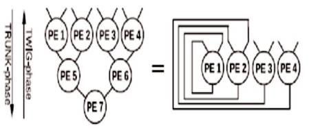
Figure 2. A Binary Tree (left, 7 PEs) is functionally equal to the unconventional Folded Tree Topology (proper, four PEs) used in this Architecture
In the digital design world, prefix operations are best known for their application in the class of carry look-ahead adders [14]. The addition of two inputs A and B in this case consist of three stages:
The outputs of the bitwise PG stage (Pi = Ai ⊕ Bi and Gi = Ai・Bi) are fed as (Pi, Gi) -pairs to the group PG logic stage, which implements the following expression:

It can be shown that, ο -operator has an identify element I =(1, 0) and is associative [11]. All these stages are explained through the example, if ο is a simple addition, then the prefix element of the ordered set [3, 1, 2, 0, 4, 1, 1, 3] is sum=15. Blelloch's procedure is used to calculate the prefix- operations and this type of addition is shown in Figure 4.
However, a binary tree implementation of Blelloch's method which is shown in Figure 3 occupies more area as it requires p = n−1 PEs for n inputs, which is not suitable for VLSI Design. In order to minimize the Area and power consumption pipelining can be traded for high throughput [10]. The concept of pipelining introduced here is to fold the tree back onto itself which leads to maximum reuse of PEs. In this method p becomes proportional to n/2 and the area is reduced to half. But strictly note that still the interconnect is reduced. Throughput decreases by using a factor of log 2(n) but since the pattern in-charge of different physical phenomena applicable for WSNs does now not exceed 100 kHz [4], this leaves enough space for this tradeoff to be made. This newly proposed folded tree topology is depicted in Figure 4(b), which is functionally equivalent to the binary tree on the left [11].
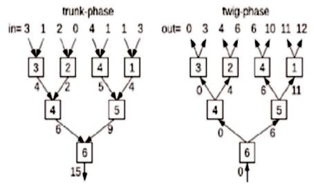
Figure 3. Blellochs Approach in Twig and Trunk Phase
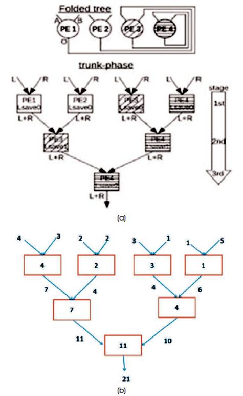
Figure 4. (a) Implications of using a Folded Tree (four4-PE folded tree proven at top): A few PEs should preserve multiple Lsave's (middle). Bottom: The trunk-section software code of the prefix-sum algorithm on a 4-PE Folded Tree, (b) Example showing Trunk Phase Operation
Due to this generic approach, algorithms are deemed to spend up to 40–60% of the time in accessing memory, making it a bottleneck. In addition, the lack of task-specific operations lead to inefficient execution, which results in longer algorithms and significant memory records maintaining. Energy consumed by this approach is high.
Now it will likely be shown how Blelloch's well-known technique for an arbitrary parallel prefix operator can be programmed to run at the folded tree. As an example, the sum-operator is used to implement a parallel-prefix sum operation on a four-PE folded tree. First, the trunk-section is taken into consideration. At the pinnacle of Figure 4(a), a folded tree with 4 PEs is drawn of which PE3 and PE4 are hatched in another way. The purposeful equivalent binary tree in the center again indicates how fact moves from leaves to root during the trunk-phase. It is annotated with the letters L and R to signify the left and right enter price of inputs A and B.
In accordance with Blelloch's approach, L is saved as Lsave and the sum L+R is handed. Note that these annotations are not global, that means annotations with the identical call do no longer always share the same real price. To see exactly how the folded tree functionally becomes a binary tree, all nodes of the binary tree are assigned numbers that correspond to the PE (1 via 4), so that it will act like that node at that stage it is shown in Figure 4. As can be seen, PE1 and PE2 are best used once, PE3 is used twice and PE is used for three instances. This corresponds to a reducing variety of lively PEs whilst progressing from level to level. The first level has all four PEs lively. The 2nd stage has active PEs they are PE3 and PE4. The 1/3 and closing degree has most effective one energetic PE that is PE4. Importantly, PE3 and PE4 should save multiple Lsave values. PE4 should preserve three (i.e.) Lsave0 via Lsave2, and PE3 maintains two (i.e.) Lsave0 and Lsave1. PE1 and PE2 maintains one: Lsave0. Finally, Figure 4 shows the practical calculations of the Trunk Phase method. This has implications towards the code implementation of the trunk phase at the folded tree. The PE application for the prefix-sum twig-segment is shown in Figure 5(a). The description column shows how records are stored, while the actual operation is given within the remaining column. The write/examine signup files (RF) columns display how incoming statistics is stored/retrieved in local RF, e.g., X@0bY approach X is stored at address 0bY, at the same time as 0bY@X masses the cost at 0bY into X. The trunksection PE software right here has three instructions, which are equal, other than the unique RF addresses that are used. Due to the fact that multiple Lsave's ought to be saved, each stage could have its personal RF deal to save and retrieve. Figure 5 shows the practical execution of twig method for the given inputs {4, 3, 2, 2, 3, 1, 1, 5}.
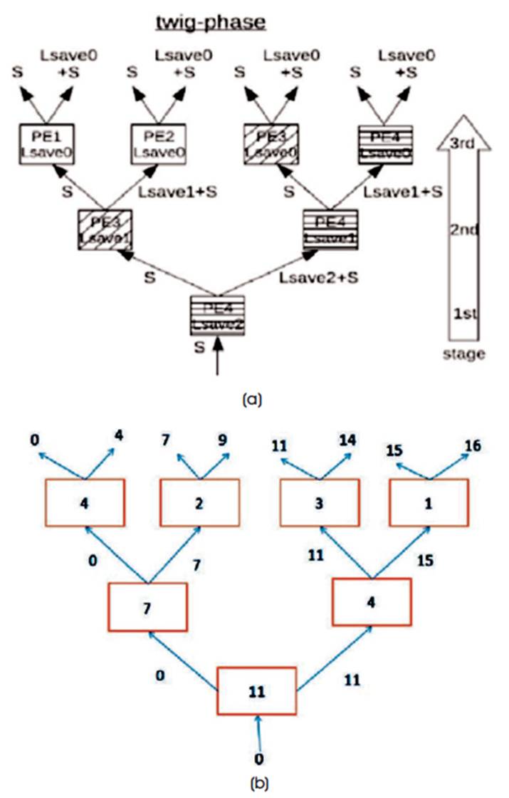
Figure 5. (a) Annotated Twig-section Graph of 4-PE Folded Tree, (b) Example showing Twig Phase Operation
If we take difference between the results in Twig section, i.e., (0,4), (4,7), (7,9), (9,11), (11,14), (14,15), (15,16). The same input values of trunk section {4, 3, 2, 2, 3, 1, 1, 5} is obtained.
The WSN nodes are simulated by using Xilinx 14.3 design suite. The simulation waveforms and synthesis results are shown in Figure 6. Here as an example base paper inputs are considered.

Figure 6. Folded Tree Approach
The simulation waveforms of trunk phase are shown in Figure 7. In order to achieve this the program was modeled by using HDL code as Verilog and verified on Xilinx14.3 Simulator tool.
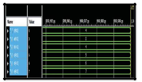
Figure 7. Trunk Phase Simulation Waveforms
Figure 8 illustrates the simulation waveforms of twig phase. To achieve this the program was modeled by using HDL code as Verilog and verified on Xilinx14.3 Simulator tool. The WSN top module is shown in Figure 9.
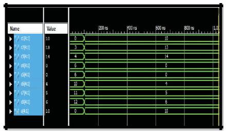
Figure 8. Twig Phase Simulation Waveforms
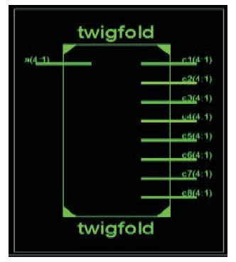
Figure 9. WSN Top Module
As it shows that the given architecture input named as a (4:1) and the output obtained is named from c1 to c8.
Register Transfer Level (RTL) shows the internal processing elements to generate the result. This RTL figure is similar to Figure 5. Figure 10 shows Twig Phase RTL Schematic.
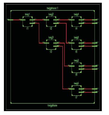
Figure 10. Twig Phase RTL Schematic
Figure 11 illustrates the design summary report of an WSN work. The design summary is related to Virtex6 FPGA prototyping Environment which is used to know the number of hardware components required to implement this design. VLSI experiments are modeled in FPGA due to the advantage that FPGA is RAM based and if any errors found in the experiment, all are modified by using FPGA and reprogrammed number of times. Also FPGA helped to reconstruct the design before implementing on ASIC. The delay is analyzed in Figure 12, that reflects the number as 1.06 ns, which is the total delay time of this experiment.

Figure 11. Design Summary
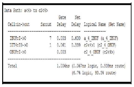
Figure 12. Synthesis Report
In this paper for efficient digital signal processing for WSN applications, the authors have used folded tree approach. In general these processors particularly for WSN nodes use parallel-prefix operations. The power consumption is minimized due to parallel-prefix-operations, reuse of binary tree as folded tree, efficient use of memory devices by using algorithms, and dataflow control elements. The Folded tree supports limited use of programmable PEs and allow to achieve low power consumption, and decreases delay.
As VLSI focus on trade-off between Area, delay, and power consumption, due to the efficient use of all the controllers and algorithms, this architecture achieves high performance WSN applications. This design is targeted to be implemented on 32 nm CMOS Technology by using Virtex6 FPGA and experimental results show that this VLSI architecture is more efficient.