[1]
Model Order Reduction (MOR) is one of the important methods to reduce the order of large scale dynamical system which come in account from previous few decades. Here, the authors inspect one of the simple and efficient methods of MOR which is Balanced Realization, and it is further divided in to two methods of MOR, among them first one is the Balanced Truncation method and second one is the Balanced Singular Perturbation Approximation method. In this paper, the authors consider three examples of real time dynamical system namely, Building Model, Partial Differential Equation Model and CD Player. Both the methods have been applied on these models and an exhaustive comparison has been made. The authors consider both the Single Input Single Output (SISO) and Multiple Input Multiple Output (MIMO) system and have applied in the above examples.
In many application areas, we need to reduce the order of large scale dynamical system in order to perform circuit simulation within a particular time limit, limited storage capacity with efficient results. A large scale system of higher dimension needs to reduce the lower dimension which can be solved by a most famous technique called MOR [32] .
Balanced realization is one of the simplest & effective model reduction scheme which is proposed first by Mooren [1]. Two different methods come under the balanced realization [20] technique i.e,
1) Balanced Truncation (BT)
2) Balanced Singular Perturbation Approximation (BSPA)
The above two methods mentioned are very much similar to each other, that of obtaining a balanced representation of a system [22]. Some of the deficiency of balanced truncation is overcome in balanced singular perturbation approximation which will be discussed in the later section.
Balanced truncation [10,11] is a time domain technique, which firstly balanced the system and then truncates (discards) the least controllable and least observable states of the original system based on the smaller Hankel singular value [12], [15]. In addition to Balanced Truncation method, a little modification takes place to stabilize the DC gains of the reduced order system to the original system is overcome in the BSPA method [2-4].
There are various model reduction techniques used for large scale dynamical systems among them, Lancozs has presented his first work under the Model Order Reduction (MDR) field in (1893-1974), where it tries to reduces the higher order matrix in its tridaigonal term [2]. Su et al. proposed an importance of smaller matrix of the larger system [7]. Moore describes the fundamental method of Model Order Reduction in the early eighties and late nineties and proposed his famous Balanced Truncation method [1]. Further, an important method is proposed by Zhou et.al [21] known as Hankel norm approximation. Sirvoich introduced a proper orthogonal decomposition method [5]. All of above methods mentioned comes under the field of control and systems theory. In 19 century, another phase of model reduction method came in existence with Krylov subspace, which introduce the first Asymptotic waveform evaluation method [6]. Now, the relationship between Pade approximation and Krylov subspace has been introduced by Freund and Feldmann [8]. Su et al. have introduced a fundamental method termed as PRIMA [7].
Internally, balanced realization is examined in the reference of model reduction technique. Balanced Singular Perturbation Approximation (BSPA) method of such realizations is not like a, balanced truncation reduction method. Here, the authors main objective is to reduce the order of large system with matching its both steady state and transient state properties. The authors consider three dynamical systems and obtained their reduced model with DC matched gain property.
For the large scale dynamical systems, the main concern is about the simplification and order reduction described by differential and difference equation corresponding to the continuous and discrete system respectively [23] .
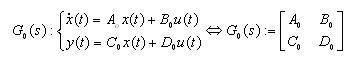
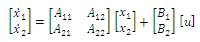
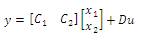
Suppose an LTI (Linear Time Invariant) continuous time is system described by:
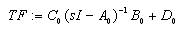
where, A , B , C , D ∈ R are matrices of different order i.e.
An×n, Bn×m, Cp×m, Dp×m . In many of the practical cases the order of the system i.e. n are very large while the system may be SISO or MIMO must satisfies m, p ∈ n. For all such type of systems, various problems occur such as, computational problem due to larger memory demand, time limitation and other conditions. One of the solution to the above problem is solved by model reduction.
The problem related to model order reduction can be
described as follows: the reduced system of order
 and the matrices
Ar , Br , Cr , Dr , of order
r x r, r x m, p x r, p x m,
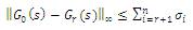
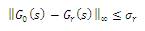
respectively, by satisfying certain properties i.e,
and the matrices
Ar , Br , Cr , Dr , of order
r x r, r x m, p x r, p x m,
respectively, by satisfying certain properties i.e,
(i) The reduction error is low and must contain an unbounded error bound.
(ii) The characteristics of the system such as stability, passivity, are protected.
(iii) The reduction technique must be estimated effectively.
Balanced Truncation (BT) method for Model Order Reduction (MOR) is one of the simple and appropriate method of order reduction technique in which the combination of two methods [16], [17] takes place. Firstly, the authors have to transform the original system into the balanced system through balanced realization and then truncates those states which have less contribution of its role in the original system [18], [19]. The algorithm used in the balanced truncation is given as follows:
Input: Consider the original system with (A, B, C, D) of order 'n' and required to reduced system of order 'r' i.e, n>>r
Output: Obtained the reduced system i.e, (Ar , Br , Cr , Dr)
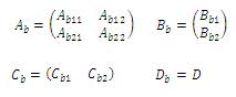
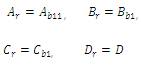
In balanced truncation method, after balancing the original system, the less controllable and less observable are truncated which causes the DC gain mismatch of obtained reduced system [29] while, instead truncating these states makes its derivative to zero or residulizes the less controllable and less observable states can yield a matched DC gain of the obtained reduced system, which is presented in the singular perturbation method [30] i.e,
The states corresponding to x1 be dominating whereas, the
states related to x2 are less controllable and less
observable. So by making derivative equal to zero for x2
states i.e,  . The resultant system
is the singular
perturbation approximation of the balanced system G(s)
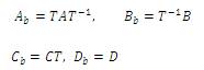
where,
. The resultant system
is the singular
perturbation approximation of the balanced system G(s)
where,
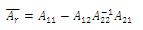
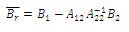
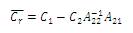
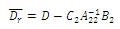
are the matrices of the reduced system and the obtained system have matched DC gain.
Algorithm of the Discussed Method
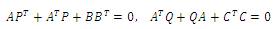
1) Solve 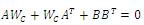 for Wc
2) Solve 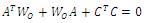 for Wo
3) Calculate the Cholesky factors,
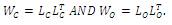
4) Calculate the SVD of Cholesky factors,

5) Find the balancing transformation matrices
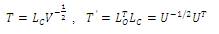
6) The balanced system obtained is given as,
7) The obtained balanced system is now divided in matrix form conformably as,
8) Truncate
to obtain the lower order system.
9) Similarity index through  criteria [24], [25],
In this part, the authors describe different examples to distinguish different balanced realization technique i.e,
i) Balanced Truncation (BT)
ii) Balanced Singular Perturbation Approximation (BSPA) We consider three models in Table 1,
a) Building Model,
b) Partial Differential Equation (PDE) Model, and
c) CD Player Model.
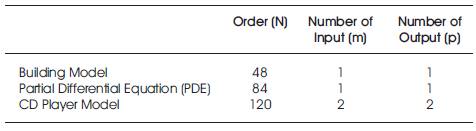
Table1. Different Real Time Model
It is an example of a SISO system with an order of 48, originally a model of the hospital of the Los Angeles University Hospital building with eight stories and linking through three sides of the surface over in x, y direction with respective rotation [9]. Hence, describing the model in polynomial system utilizing the 24 states:
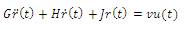
where u(t) is the input and the model is described by canonical state space form of order 48.
Consider the Partial Differential Equation (PDE) [9]
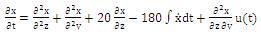
where, x is related to 't','v','z', which represents time,
vertical
and horizontal positions respectively. The points (0,0) and
(1,1) on the diagonal of the square are taken as the
boundaries points. The x will satisfy the boundary condition.
Now the model is made to sample on the basis of the gird
having points nv x nz with centered difference
approximations. The function  interlinked with input
vector consists of random elements. To make the system
simpler, the authors considered both the input and output
vector equal to each other.
interlinked with input
vector consists of random elements. To make the system
simpler, the authors considered both the input and output
vector equal to each other.
In this model, the main controlling element is used to control the speed of the disc focused by a laser point to the rotating pits of a disc. A swinging arm is there, upon which a lens is placed through the two horizontal leaf springs. Because of the rotating nature of the arm placed over the horizontal plane, it is responsible to take measures of disc (spiral-shaped) tracks, and for the imaging of the disc suspended lens. The several irregularity in the disc and in the other arrangement i.e, disc is not completely flat, imperfectness in the shape of the disc, all of the above problems can cause a difficulty to design the cost permissible controller through, which we can control the model from shocks and sluggishness.
For Building model of 48 orders, the authors first apply the BT method and obtained the reduced model of order 18, which consists of larger Hankel singular value and truncate the remaining states corresponding to smaller Hankel singular value.
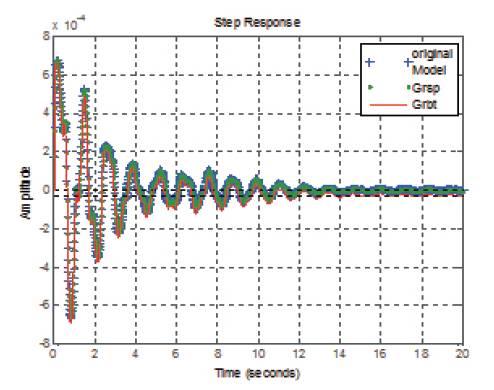
Figure 1. Compared the Step Response of Building Model with BT and BSPA Method
Figure 1 describes the simulation results based on BT and BSPA method with stabilizing DC gain (Steady state) of the reduced order system i.e, eliminate the steady-state deviations and preserve the dynamic behaviors.
Original System Order - 48
Reduced System Order - 18
The authors compute the errors [27] between the original model and the reduced model by two methods i.e. Infinity Error and Integral Square Error (ISE) as shown in Table 2.
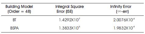
Table 2. Error Analysis for BT and BSPA Method
The second example the authors consider is a PDE model of order 84, which is a SISO system and reduces the original system by using BT and BSPA method and comparing their step response, it results with stabilizing its DC gain to match the steady state response of the reduced system with the original system.
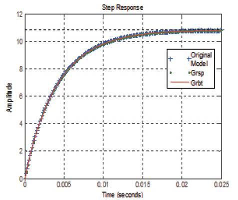
Figure 2. Compared the Step Response of PDE Model with BT and BSPA Method
Figure 2 describes the simulation results based on BT and BSPA method with stabilizing DC gain (Steady state) of the reduced order system i.e. eliminate the steady-state deviations and preserve the dynamic behaviors.
Original System Order - 84
Reduced System Order - 04
The authors compute the errors between the original model and the reduced model by two methods i.e. Infinity Error and Integral Square Error (ISE) as shown in Table 3.
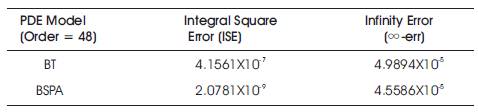
Table 3. Error Analysis for BT and BSPA Method
The last example i.e. CD Player is a MIMO system of order 120. Previously, all of the real time examples considered are SISO system and both the methods are applied and tested for the SISO system. Now,it is applied to the MIMO system and analysis its results by using both the BT and BSPA method.
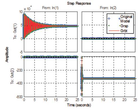
Figure 3. Compared the Step Response of PDE Model with BT and BSPA Method
Figure 3 describes the simulation results based on BT and BSPA method with stabilizing DC gain (Steady state) of the reduced order system i.e, eliminate the steady-state deviations and preserve the dynamic behaviors.
Original System Order - 120
Reduced System Order - 08
The authors compute the errors between the original model and the reduced model by two methods i.e. Infinity Error and Integral Square Error (ISE) as shown in Table 4.
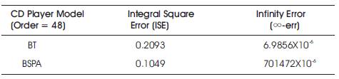
Table 4. Error Analysis for BT and BSPA Method
In this paper, the authors have considered three examples of real time dynamical system namely, Building Model, Partial Differential Equation (PDE) Model and CD Player model to obtain their reduced order model. BT and BSPA has been applied successfully to obtain their Approximation. The closeness of the approximation has been measured through the ISE and ∞ -error as performance index. The value obtained through these indexes confirms the closeness with the original system. The methods have been extended to MIMO case also.